Symplectic topology
Symplectic Topology
Math 705
Notes by Patrick Lei,
Spring 2020
Lectures by R. İnanç Baykur
University of Massachusetts Amherst
Disclaimer
These notes were taken during lecture using the vimtex package of the editor neovim. Any errors are mine and not the instructor’s. In addition, my notes are picture-free (but will include commutative diagrams) and are a mix of my mathematical style (omit lengthy computations, use category theory) and that of the instructor. If you find any errors, please contact me at plei@umass.edu.
1 January 21
1.1 Course Description
This is an introductory course on symplectic topology, along with its connections to differential, complex algebraic, and contact geometry and topology.
1.2 Organization
İnanç passed around a syllabus. Prerequisites for this course are smooth manifolds, some algebraic topology (cohomology), and complex analysis. Because this is a second year graduate course, we are expected to read any missing background on our own. Grading will be based on homework and a final presentation. We will cover the first four topics on the syllabus and do some of the last four. Finally, İnanç may add more geometry to the course.
1.2.1 Notational conventions
We will denote finite dimensional real vector spaces over by and smooth manifolds by .
1.3 Basic Notions
Definition 1.1.
A symplectic form (or a symplectic structure) on a vector space is a nondegenerate alternating bilinear form .
Definition 1.2.
A symplectic form (or symplectic structure) on a smooth manifold is a differential form which is closed and everywhere nondegenerate.
Remark 1.3.
A fundamental question to ask is when a manifold admits a symplectic structure. We will see that symplectic structures exist only on even-dimensional manifolds. Saying more is an extremely difficult problem, although we can say that symplectic manifolds admit an almost complex structure and are orientable. Uniqueness up to both symplectomorphism and deformation is also very difficult.
Example 1.4.
Let with coordinates . Then we can define a form
where
Checking that is a nondegenerate alternating bilinear form is easy. Later we will see that this is the only symplectic vector space.
Example 1.5.
Consider with coordinates . Now consider the form
Checking that this form is closed and nondegenerate is easy. We can also define the form on , where the form becomes
Note that the requirement that symplectic forms are closed is a subtle condition. If we multiply by a general function, the resulting form will not be closed. Recall that smooth manifolds are locally Euclidean. We can require our transitions to lie in the symplectic group, and later we will show that this definition of a symplectic manifold is equivalent to the one we gave today.
For a general manifold , we want to associate linear spaces to it.
Definition 1.6.
A vector bundle over is a symplectic vector bundle if there exists a smooth section of such that is a symplectic vector space for all .
Example 1.7.
For a symplectic manifold , the tangent bundle is a symplectic vector bundle.
Remark 1.8.
Observe that if the tangent bundle is symplectic, then the manifold is not necessarily symplectic.
1.4 Symplectic Linear Algebra
Definition 1.9.
For symplectic vector spaces, a linear symplectomorphism is an isomorphism of vector spaces such that . They and are symplectomorphic.
The usual definition of orthogonal complements carries over and will be denoted for a subspace .
Lemma 1.10.
Let be a symplectic vector space.
- 1.
is an isomorphism .
- 2.
.
- 3.
.
- 4.
The following are equivalent:
- (a)
is a symplectic subspace of ;
- (b)
is symplectic;
- (c)
;
- (d)
.
- (a)
Proof.
- 1.
This part is equivalent to nondegeneracy.
- 2.
Use a rank-nullity argument to note that maps to the annihlator of under the isomorphism .
- 3.
Clearly . Then use the dimension result.
- 4.
Clearly a) implies c) and c) and d) are equivalent. Finally, it is easy to see that d) implies a). Finally equivalence of b) to the rest is easy.
□
Theorem 1.11 (Symplectic Basis).
For any symplectic vector space , there exists a basis such that
called a symplectic basis for .
2 January 23
2.1 More Basic Linear Algebra
Last time we stated the following:
Theorem.
For any symplectic vector space , there exists a basis such that and any other pairing is zero.
Proof.
We will induct on the dimension of the vector space. For , take any nonzero . Then by nondegeneracy, we can find a desired . Then we simply use Lemma 1.4.2, note that span a symplectic subspace of , and apply the inductive hypothesis to . Because are orthogonal to the symplectic basis for , we are done. □
Corollary 2.1.
Any symplectic vector space is symplectomorphic to .
Proof.
Observe that
Define our morphism in the obvious way:
Then it is easy to check that
□
Corollary 2.2.
A skew-symmetric on is symplectic iff .
Proof.
If is symplectic, then there exists a symplectic basis , and . In the other direction, if is degenerate, there exists such that for all . Then we can complete to a basis by , and here , so . □
2.2 Compatible Complex Structures and Inner Products
Tailoring the class to the audience, İnanc will return to the theme of the three geometries: Riemannian, symplectic, and complex. We will see that symplectic geometry lies between the other two geometries (every manifold admits a metric, complex algebraic structures are very rare).
The group of linear symplectomorphisms of is denoted by .
Definition 2.3.
A real matrix is symplectic if , where was defined in Example 1.3.4. The group of such matrices is .
By Corollary 2.1.1, we see that .
Definition 2.4.
A complex structure on a real vector space is an automorphism such that . Then is a complex vector space with the definition .
Then .
Definition 2.5.
If is a symplectic vector space, a complex structure is called -compatible if for all and for all nonzero .
Let be the space of -compatible complex structures on with topology inherited from (here endomorphisms are taken in ). This space will turn out to be contractible, but first we need to show that it is nonempty. This is true because is compatible with the standard form. The taming property is also easy to check.
Recall that an inner product on a real vector space is a nondegenerate symmetric positive-definite bilinear form . Here, .
Definition 2.6.
A Hermitian structure on is an inner product on such that for all .
Remark 2.7.
If is any inner product on , then is Hermitian.
Remark 2.8.
if and only if is a Hermitian inner product.
Proof.
Note that iff iff . In addition, iff clearly. □
Example 2.9.
The standard symplectic form, the matrix , and the standard inner product on is a compatible triple.
Theorem 2.10.
is contractible.
Proof is left to the next lecture because it will take too long for the rest of this lecture.
Remark 2.11.
The analogous result for almost complex structures on symplectic manifolds will allow us to discuss Chern classes on symplectic manifolds.
Now let be the space of inner products on . We can define varying smoothly in .1
Remark 2.12.
Given a complex vector space and a compatible inner product , we can derive a symplectic structure on for which is -compatible by .
Proof of this fact is left to the reader. Exercises will be assigned nect time.
3 January 28
3.1 A Big Theorem
Last time we stated the following:
Theorem.
is contractible.
Proof.
Let be the space of inner products on with topology given by choosing a unitary basis for . We identify with the set of symmetric positive-definite matrices. Under this identification, becomes a smooth manifold. We will show that retracts onto . Because is convex, it is contractible.
Consider the automorphism given by Now observe that . Therefore the adjoint of is . Then we write , which is symmetric and positive definite. We now have
Then we can write , which is symmetric and positive definite. Now set .1
We will show that . First note that and commute (because and commute). Therefore preserves the eigenspaces of . This gives
Moreover, is self-adjoint and is skew-adjoint, so is skew-adjoint. Also commutes with .
Now we show -compatibility. The first condition is just
The taming condition is simply
because all eigenvalues of are positive. This gives us a map which can be checked to be smooth. We can define the right inverse by . This can also be checked to be smooth. It is easy to see that if , then the polar decomposition gives , so is a retraction. Therefore is homotopy equivalent to . □
Lemma 3.1.
Let be symmetric. Then the following are equivalent:
- 1.
is positive definite.
- 2.
All eigenvalues of are positive.
- 3.
, where is orthogonal and is diagonal with positive entries.
- 4.
for some nonsingular .
3.2 More Compatibility
Definition 3.2.
We call on a compatible triple if .
Observe that any two determine the third. Moreover, we have seen that we can complete two of them to a compatible triple if:
- •
For , is -compatible.
- •
For , is -compatible.
- •
There are no conditions on to obtain a .
Exercise 3.3.
Let be a compatible triple on with . Show that
- (a)
.
- (b)
For any subspace , .
Note that for standard , the automorphism groups overlap as .
Theorem 3.4.
Any two of the above groups intersect as .
Proof.
Recall that
- 1.
iff ;
- 2.
iff ;
- 3.
iff .
It is not hard to see that any two imply the third. For example, if we have the first two, then
□
How about the spaces of these structures? We denote the space of symplectic structures by , the space of complex structures by , and the space of inner products by . Note that acts transitively on with stabilizers . Because is a Lie group acting transitively on a smooth manifold, every stabilizer is closed. Then a quotient of a Lie group by a closed subgroup is a smooth manifold.
Therefore we may consider the spaces . These spaces are exactly , respectively. Thus they are smooth manifolds.
Exercise 3.5.
Compute their dimensions. Also compute their for .
Theorem 3.6.
.
Proof.
If is -compatible, let . This is a hermitian structure. For a unitary basis of , we have a symplectic basis . Then define the map
which is a symplectomorphism. Set by . This is an isomorphism. □
4 January 30
4.1 Homework Exercises
İnanç will post homework later, and it will be due in approximately two and a half weeks.
Exercise 4.1.
Find . In other words, find a complex structure not compatible with the standard symplectic form.
Exercise 4.2.
Find . In other words, find a matrix which is not symplectic.
Here are some facts that will be helpful on the homework.
Proposition 4.3.
Let . Then
- 1.
;
- 2.
;
- 3.
is an eigenvalue with multiplicity iff is as well;
- 4.
If is an eigenvalue of , then it has even multiplicity;
- 5.
If are eigenvectors for with , then .
- 6.
If is symmetric and positive-definite, then for any .
Proof.
- 1.
Note that preserves the symplectic form . Therefore it preserves the volume form and the orientation.
- 2.
We see .
- 3.
Because , then , so have the same eigenvalues. Then if if an eigenvalue of with multiplicity , we have , so . Thus is an eigenvalue of and therefore of .
- 4.
must have even multiplicity to ensure that has determinant .
- 5.
Note that . Because , we must have .
- 6.
Let be an eigenspace of . This is an eigenspace for under . By the above, we if , then are orthogonal under . In addition, by the previous, it is easy to see that preserves on the eigenbasis. □
4.2 Subspaces of Symplectic Vector Spaces
For a given symplectic manifold, there are four kinds of submanifolds we will describe. Two of them are important, and the other two will allow us to reduce to the first two.
Let be a subspace of the symplectic vector space . Recall that is symplectic if .
Definition 4.4.
is
- •
isotropic if ;
- •
coisotropic if ;
- •
Lagrangian if .
Example 4.5.
Consider with the standard form with basis . Then
- •
The spaces are symplectic;
- •
The spaces are isotropic;
- •
The spaces are coisotropic;
- •
The spaces are Lagrangian.
Proposition 4.6.
Let be a synplectic vector space of dimension .
- 1.
Any line is isotropic;
- 2.
Any hyperplane is coisotropic;
- 3.
Any isotropic subspace is contained in some Lagrangian subspace;
- 4.
Any coisotropic subspace contains some Lagrabgian subspace;
- 5.
preserves the four types of subspaces.
Proof.
- 1.
is alternating.
- 2.
is a line, so it is isotropic. Thus .
- 3.
If is isotropic but not Lagrangian, then there exists . Then set . This is clearly also isotropic. Repeat until has dimension .
- 4.
is isotropic, so use the above to find . Then .
- 5.
We show that . If , then , so . Therefore, , so . Thus Because the two spaces have the same dimension, they are equal. □
Proposition 4.7 (Symplectic Reduction).
Let . If is isotropic (resp. coisotropic), then (resp. ) is symplectic.
Proof.
Let . Then for any . Therefore is defined on equivalence classes modulo . Therefore we only need to check nondegeneracy. If is such that for all , then . Therefore is nondegenerate on . □
Note that symplectic and Lagrangian subspaces are good for constructing new symplectic spaces and defining symplectic invariants (Floer homology, Gromov-Witten invariants). When we switch to discussing manifolds, we will see that Lagrangian submanifolds are hard to find, while symplectic submanifolds are easy to find. We will only want to consider some symplectic submanifolds.
Define to be the space of Lagrangian subspaces of and to be the space of Lagrangian subspaces of , the Lagrangian Grassmannian.
Proposition 4.8.
.
Sketch.
For , choose an orthonormal basis with respect to . Set
Therefore, , where is the span of the first standard vectors. Also, note is unitary. Conversely, for all , clearly is also Lagrangian. Set by . We can check that this is an isomorphism. Next time we will say some things about . □
5 February 4
5.1 Linear Algebra, Conclusion
Last time we discussed the Lagrangian Grassmannian .
Remark 5.1.
- 1.
. In addition, the determinant map is a fibration with fiber . Then, the projection onto the first colume is a fibration with fiber , so by the homotopy long exact sequence, we have an exact sequence
This tells us that . In particular, . Now going back to , then we use the homotopy LES to obtain
so .
- 2.
By the universal coefficient theorem, . The generator is called the Maslow index . For a loop in , we then define the Maslow index of as .
5.2 Symplectic Vector Bundles
Recall that a symplectic vector bundle over a manifold is a real vector bundle with a section of such that is a symplectic vector space for all . Then two symplectic vector bundles are isomorphic if there exists an isomorphism such that .
Example 5.2.
If is symplectic, then is a symplectic vector bundle. In addition, the pushforward of a symplectomorphism is an isomorphism of symplectic vector bundles.
Remark 5.3.
Given any vector bundle , we can define a symplectic vector bundle on the Whitney sum by
This is clearly bilinear, antisymmetric, and non-degenerate.
Definition 5.4.
A complex vector bundle over a manifold is a real vector bundle with a section of such that is a complex vector space for all .
We say two complex vector bundles are isomorphic if there exists a vector bundle isomorphism such that .
Example 5.5.
Let be a complex manifold of dimension . Then define the usual multiplication by on . Now we need to see if this is globally defined. To do this, we simply compute on two charts and then use the Cauchy-Riemann equations. This is left to the reader.
Remark 5.6.
Given any vector bundle , we can define a complex vector bundle on .
Definition 5.7.
If is a symplectic vector bundle over , a complex structure on is called -compatible if for all .
Denote by the space of -compatible complex structures on with the topology inherited from .
Definition 5.8.
A Hermitian structure on is a -compatible inner product (at every ).
Remark 5.9.
- 1.
We can construct a Hermitian inner product from any inner product as before.
- 2.
The space of Hermitian structures is convex.
- 3.
if and only if is Hermitian.
Theorem 5.10.
is nonempty and contractible.
Proof.
Define the retract by using the map in Theorem 2.10 pointwise. In a local trivialization of , we can see that is smooth. □
Now we will consider chart transitions for . Denote the chart for the local trivializations by with trivializations .
| Type | Group |
|---|---|
In each special case, the structure of the bundle can be reduced. Note here that we also have the two out of three property for reduction to as before. We will illustrate this by checking the case. We simply note that , which admits a symplectic basis. Therefore we have a symplectic trivialization of . Therefore, locally we have an isomorphicm to . Therefore we have reduction of the structure to .
Now suppose the structure of can be reduced to . Then the corresponding is -compatible.
Theorem 5.11.
- 1.
Let be a symplectic vector bundle and . Then .
- 2.
Let be symplectic vector bundles and . Then if and only if .
6 February 6
6.1 Proof of Theorem 5.11
İnanç will post the homework tonight. Last time we stated Theorem 5.11, which is reproduced below.
Theorem.
- 1.
Let be a symplectic vector bundle and . Then .
- 2.
Let be symplectic vector bundles and . Then if and only if .
Proof.
- 1.
First, note that for any structure group of a real vector bundle, there exists a classifying space with a contractible universal -bundle . In particular, -bundles are classified by homotopy classes of maps . In other words, represents the functor on the homotopy category.
Now use the homotopy LES of the fibration to obtain isomorphisms . In particular, the inclusion induces an isomorphism on all . By Whitehead, this is a homotopy equivalence. Therefore . Therefore for any , this determines , which can be homotoped to , which reduces uniquely to a -bundle.
- 2.
By the previous, isomorphism as -bundles implies isomorphism as -bundles. Now consider the inclusion . This is a homotopy equivalence (use Gram-Schmidt to deform any loop into ). By similar arguments as above, two -bundles are isomorphic iff they are isomorphic as -bundles. This concludes the proof. □
Remark 6.1.
Note that this allows us to determine whether two symplectic vector bundles are isomorphic by comparing their Chern classes.
6.2 Vector Bundles, Continued
Let be a subbundle of the symplectic vector bundle .
Definition 6.2.
The symplectic complement of is
Definition 6.3.
We define the vector subbundle to be
- •
symplectic if is the zero section of ;
- •
isotropic if ;
- •
coisotropic if ;
- •
Lagrangian if .
Many previous results on subspaces carry over to subbundles.
Proposition 6.4.
Let be a subbundle of the symplectic vector bundle .
- 1.
If is symplectic, , then there exists extending .
- 2.
If is Lagrangian, , then .
Proof.
- 1.
If is symplectic, then so if . Therefore there exists . Then we have , so we write . All properties of an -compatible complex structure follow from the orthogonal decomposition of .
- 2.
Let be a compatible inner product for . Then . To see this, note that , which is the same complex structure as . □
6.3 Compatible Triples on Manifolds
Let with symplectic structure , complex structure , and inner product . When only defined on , then is an almost symplectic structure and is an almost complex structure. In this course, we will focus on the case when is a true symplectic structure on . We define the following spaces:
- •
the space of symplectic structures on ;
- •
the space of almost complex structures on ;
- •
the space of almost complex structures on ;
- •
the space of compatible almost complex structures.
Definition 6.5.
Now let be a submanifold of . Then is a subbundle of , and we call
- •
symplectic if is symplectic;
- •
isotropic if is isotropic;
- •
coisotropic if is coisotropic;
- •
Lagrangian if is Lagrangian;
Note that is symplectic iff is a symplectic manifold. In addition, note that must be even dimensional and the nomal bundle . Also, note that is Lagrangian iff .
Definition 6.6.
For a submanifold of , we call , we call -holomorphic if , which happens iff is an almost complex structure on .
Remark 6.7.
Our results about symplectic vector bundles carry over to . In particular, is nonempty and contractible.
Proposition 6.8.
Let be a submanifold of .
- 1.
If is symplectic, then is -holomorphic for some ;
- 2.
If is -holomorphic for any , then is symplectic.
Proof.
- 1.
This is (mostly) just the first part of Proposition 6.4. However, we must extend from to all of . First we take a compatible metric, extend it by a partition of unity, and then use the retract to find a compatible .
- 2.
Note . Therefore , so is symplectic.
□
Exercise 6.9.
Find a symplectic submanifold of that is not -holomorphic.
7 February 11
7.1 Obtaining Compatible Triples
| Input | Condition | Output | Integrable? |
|---|---|---|---|
| is -compatible | metric | flat? | |
| is Hermitian | almost symplectic | closed? | |
| none | almost complex | integrable? |
- 1.
This is the same as local flatness. By a theorem of Bieberbach, all compact flat manifolds are finitely covered by tori.
- 2.
This is the same as . If is a complex structure and is Hermitian, then is a fundamental -form. The Goldberg conjecture states that if is Einstein, then .
- 3.
By a theorem of Newlander and Nirenberg, there exists a complex structure on inducing if and only if the Nijenhuis tensor .
Definition 7.1.
The Nijenhuis tensor of is defined by
Exercise 7.2.
- 1.
If the map is -holomorphic for all , then .
- 2.
Check that is a tensor.
- 3.
If has dimension , then .
7.2 Complex Structures
Definition 7.3.
is a Kähler manifold when is integrable.
Example 7.4.
Any a closed oriented surface of genus is a Kähler manifold. To see this, take . Then it is easy to see that is bilinear, skew-symmetric, nondegenerate, and closed. Now let , so is a compatible triple on . But any almost complex structure on a surface is integrable by Exercise 7.2, so we are done.
Now let be an almost complex structure on . Take the complexified vector bundle . Then extends linearly to as
Then we can see that , so the eigenvalues are . Then we can define as the eigenspaces of . Therefore we obtain an isomorphism
In addition, we can write . Then we have
Therefore we have
We want to define a differential that describes this structure. We can define by
and then define analogously.
Now if , then we must have . This allows us to define Dolbeaut cohomology.
Suppose is a complex structure on . Then in a local chart , we have coordinates and we can write . In addition, . Writing a form locally, we will see that .
Remark 7.5.
For any almost complex structure on , if , then is integrable.
Theorem 7.6 (Newlander-Nirenberg).
Let be an almost complex structure on . Then the following are equivalent:
- 1.
is induced by a complex structure on ;
- 2.
;
- 3.
;
- 4.
.
Now suppose be Kähler. Then what can we say about ?
- •
is a closed form over ;
- •
If , then and ;
- •
Computing , we will see that is a -form.
- •
.
8 February 13
Recall that there will be no class next Tuesday. Last time we began the discussion of Kähler forms.
8.1 Kähler Forms Continued
Recall from last time that Kähler forms are of type . Also recall that locally we have
In order to express the coefficients as a metric, we can rewrite
| (8.1) |
Then the matrix is a Hermitian matrix. In particular, the volume form is locally
Proposition 8.1.
Now let be a compact complex manifold of dimension with complex structure . Then the following are equivalent:
- 1.
is a Kähler form on ;
- 2.
is a and -closed -form locally given by (8.1) with coefficient matrix given by a Hermitian positive-definite matrix.
Proof.
We did one of the directions above. In the other direction, observe that is locally given by for a Hermitian positive definite matrix. Thus is nondegenerate. In addition, is clearly -compatible because it has type . □
Example 8.2.
is Kähler with complex structure .
Example 8.3.
Consider . Recall the standard complex atlas for . Let be the induced complex structure on . Then there exists a symplectic form , the Fubini-Study metric, on compatible with .
Proposition 8.4.
Any complex submanifold of a Kähler manifold is Kähler.
First Proof.
Let be a complex manifold of dimension and be a complex manifold of dimension . Then locally at , we have charts for such that . If is a Kähler form on , then locally we have
In particular, it is easy to see that the coefficient matrix is Hermitian and positive definite. Finally, is a -closed -form, so is as well. □
Second Proof.
Note that is a -holomorphic submanifold of . By Proposition 6.8, is also a symplectic submanifold of . Therefore is symplectic and compatible with , which is already integrable. □
8.2 Some Algebraic Geometry
Thus we have proven the following corollary, which tells us that any smooth affine or projective complex algebraic variety is Kähler.
Theorem 8.5.
Any complex submanifold of or is Kähler.
Remark 8.6.
We will state some facts from complex algebraic geometry in context for culture.
- 1.
Many complex submanifolds of are not affine, e.g. .
- 2.
By Chow’s theorem (1949), any closed complex submanifold of is algebraic.
- 3.
The Kodaira embedding theorem (1960s) states that a closed Kähler manifold is algebraic if and only if is integral.
Proposition 8.7.
In particular, any compact complex curve is projective.
Proof.
On equipped with complex structure , take any -compatible metric . Then set . Then is symplectic. Therefore is a Kähler form on compatible with . Now suppose that
Because any nonzero real multiple of a Kähler form is still Kähler, then is the desired integral form. □
Remark 8.8.
Not all compact Kähler surfaces are projective. In complex dimension , Kähler manifolds become projective after deforming the complex structure. In dimension at least , there exist compact Kähler manifolds (due to Voisin) that are not even homotopy equivalent to a projective variety.
Theorem 8.9 (Gromov’s Embedding Theorem).
Let be a closed symplectic manifold. If is integral, then there is a symplectic embedding of into for some high enough .
Remark 8.10.
İnanç says this theorem is conceptually nice, but he does not know any use for the result.
Example 8.11.
Let . Then .
Now let be a hypersurface of degree in . Then , and is a K3 surface (use the adjunction formula).
8.3 Stein Manifolds
Let be a complex manifold of dimension and let be a proper, strictly plurisubharmonic function on .
Definition 8.12.
A function is structly plurisubhamonic if on each complex chart, is positive-definite.
In this case,
is a Kähler form on , and we say is a Stein manifold, where is the Kähler potential.
9 February 20
9.1 Stein Manifolds Continued
Today’s lecture will be slower than usual. Last time we defined Stein manifolds , where is strictly plurisubharmonic. It is easy to see that is closed and real. Also, .
Example 9.1.
Choose and . Then we can check that is the identity matrix. Then we can also see that
is the standard form.
Thus every complex submanifold of is a Stein manifold.
Theorem 9.2 (Remmert Embedding Theorem (1956)).
Let be a Stein manifold. Then there exists a proper holomorphic embedding of into for some .
Corollary 9.3.
Stein manifolds do not have compact complex submanifolds of positive dimension. In particular, they are never compact.
Theorem 9.4 (Behnke-Stein (1958)).
Every connected non-compact complex curve is Stein.
9.2 Topological Properties of Kähler Manifolds
Theorem 9.5 (Hodge).
On a compact Kähler manifold , the Dolbeaut cohomology groups satisfy the Hodge decomposition
In addition, we have an isomorphism
Theorem 9.6 (Serre Duality).
For any complex manifold , we have .
Remark 9.7.
We obtain the Hodge numbers , which are traditionally arranged in the Hodge diamond, which has symmetry given by the Hodge symmetry and Serre duality.
Example 9.8.
Consider a curve of genus . Then the Hodge diamond is
Example 9.9.
The Hodge diamond of is
Example 9.10.
The Hodge diamond of is
Example 9.11.
The Hodge diamond of is
Example 9.12.
Consider the Hopf surface, which is the quotient of by the action of acting by powers of . This is a biholomorphic, free, and properly discontinuous action. Up to diffeomorphism, our surface is . Note that the second cohomology vanishes, so the surface is not Kähler. The Hodge diamond of the Hopf surface is
Remark 9.13.
The odd Betti numbers of compact Kähler manifolds are even. The even Betti numbers are positive because is closed but not exact. In fact, any symplectic manifold has nonvanishing even cohomology. In particular, is always positive.
9.3 Complex and Symplectic Structures on -Manifolds
Let be a closed, connected, oriented, smooth -manifold. The equivalences will be orientation-preserving diffeomorphisms. We will see that for complex surfaces, Hodge numbers depend only on the topological type of the oriented manifold.
Recall the Euler characteristic and the signature . The signature of the manifold is the signature of the quadratic form , called the intersection form.
Remark 9.14.
If are homotopy equivalent, then they have the same intersection form. Also, if is with the opposite orientation, then . Third, if , then .
Theorem 9.15 (Whitehead).
If are simply-connected and , then .
Theorem 9.16 (Freedman).
If are simply connected, are either both smoothable or both not smoothable, and , then .1
Example 9.17.
The intersection form of is and the intersection form of is
10 February 25
10.1 Complex Structures in Dimension 4
Recall that for Kähler surfaces, the Hodge numbers depend only on the top type of the oriented manifold.
Theorem 10.1 (Kodaira-Siu (1981)).
Let be a compact complex surface. Then is Kähler if and only if is even.
Remark 10.2.
The existence of an almost complex structure is a purely homotopy-theoretic problem.
Theorem 10.3 (Wu’s criterion).
Let be a closed oriented -manifold. Then admits an almost complex structure if and only if such that and .1
Example 10.4.
On , the second cohomology vanishes, so . This implies , but . Therefore admits no almost complex structure.
Example 10.5.
On , note that , so . Clearly satisfies the second part of Wu’s criterion, so admits a complex structure. However, the two almost complex structures are not equivalent.
Example 10.6.
Consider . Here, if , then . However, , so there is no almost complex structure.
Example 10.7.
Now consider the manifold . Then we have , so if we write , then . However, , which is not a sum of two squares. Therefore there is no almost complex structure.
Remark 10.8.
We see that orientation reversal and connected sum are not almost complex operations. Therefore, they are also not symplectic operations.
Example 10.9.
Consider the connected sum . Here we see that . In addition, are all odd, so this manifold does admit an almost complex structure.
10.2 Symplectic Structures in Dimension 4
10.2.1 Seiberg-Witten Invariants
These come from a certain system of differential equations on which come from physics. The solutions yield a very nice moduli space under facorable conditions for each : If and admits an almost complex structure, then for all but finitely many . Then is a compact oriented manifold with dimension
For with , then we can assign the signed count of points in . If , we need an additional choice. Then this defines the Seiberg-Witten invariant . Then for any with is called a Seiberg-Witten basic class.
Remark 10.10.
Here are some fundamental results:
- 1.
The Seiberg-Witten invariant is invariant under orientation preserving diffeomorphisms.
- 2.
(Vanishing Theorem). If , with for , then .
- 3.
(Taubes). If is symplectic with , then there exists a particular such that . In fact, for any -compatible .
Theorem 10.11 (Diversity).
There exist infinitely many closed, connected, oriented maniflds of dimension . Smooth manifolds in each subclass are depicted below.
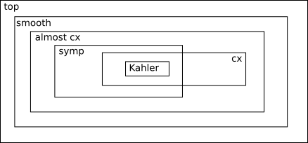
Proof.
First, Freedman’s -manifold is not smoothable. Then has no almost complex structure. Third, is not symplectic by Taubes and not complex by Kodaira-Siu. Fourth, admits a complex structure, but is not symplectic or Kähler. Fifth, the Kodaira-Thurston manifold is complex and symplectic, but not Kähler. □
Remark 10.12.
Infinitely many examples in each subclass can be obtained by blowups .
Example 10.13 (Kodaira-Thurston Manifold).
Let act in with coordinates , where increases the th component by for , while . This is a free and properly dicontinuous action, so is a smooth manifold. Then is the universal cover of . Then we see that all commute exept for . Therefore , so . Therefore cannot be Kähler.
11 February 27
Exercise 11.1.
Let be a finite unbranched cover. Show that if is symplectic, almost complex, complex, Kähler, projective, or Stein, then so is .
11.1 Kodaira-Thurston Manifold
Recall the definition of the Kodaira-Thurston manifold as a quotient of by a discrete group from last time.
Remark 11.2.
We may obtain as a -bundle over the torus.
To see this, note that we can project onto the first two coordinates. This is a map , where acts by shifts. To compute the fiber, note that , where identifies and . Thus the fiber is a torus. The action of becomes nontrivial monodromy.
To see the monodromy, note that if we move in the -direction in the base, identifies with . However, in the -direction, identifies with .
This gives us a description of the monodromy by the matrices .1
Theorem 11.3 (Thurston (1976)).
The manifold is symplectic.
Proof.
Choose the standard symplectic form . Next we can see that for all . The only one we need to check is , and we see that
because . Therefore each is a symplectomorphism, so is a symplectomorphism of . Thus is a covering with symplectic deck transformations. Thus there is an induced symplectic form on . □
Theorem 11.4 (Kodaira (1969)).
The Kodaira-Thurston manifold is complex.
Proof.
Let . Then this gives a -invariant basis for . The only one we need to check is with , and we see that
Then note that are all closed, but . Then the dual basis
is a -invariant basis for the Lie algebra of vector fields on . To see this, we only need to check , and we see
as desired. Now define . Then we see that
Similarly, note that
Here we use the fact that all commutators vanish besides . Therefore is a complex structure on . In addition, the -invariant basis for vector fields on descends to a basis for vector fields on . Also, descends to an integrable almost complex structure on . □
Corollary 11.5.
The Kodaira-Thurston manifold is complex and symplectic but not Kähler.
Remark 11.6.
The -invariant basis descends to . In addition, the symplectic form descends to the form
11.2 Algebraic Topology of
For simplicity, we will drop the bars. Recall that , while . Also, note that . Then recall that and note that . Therefore, we obtain .
We will write a basis for each cohomology and write the intersection form. We have
and
Next, we see that and .
Finally, we can see the intersection form is given by
From this, we see that , so .
12 March 3
Note: I was not here on this day. Notes were provided by Arthur Wang.
12.1 Topology of Complex Manifolds
We will answer the following question:
Question 12.1.
Are there any differential topological constraints for a symplectic -manifold to admit a complex structure?
Recall that all symplectic manifolds have an almost complex structure. Also, they have positive .
Theorem 12.2 (Kodaira-Siu).
If is a compact complex surface, is Kähler if and only if is even.
We can consider with even first Betti number. Then if is complex, then it is Kähler. However, there are no constraints that come from Hodge theory. There are, however, more constraints from differential topology.
Theorem 12.3 (Hard Lefschetz).
For the Kähler form, is an isomorphism for all . Here sends to .
This gives us Serre duality on Dolbeault cohomology.
Remark 12.4.
All triple Massey products on Kähler are zero: Let with . Then
is defined as follows:
Take with , so and . Then
There is a constraint from algebraic topology. Not all finitely presented groups are fundamental groups of Kähler manifolds. For example, if the abelianization of has odd rank, then is not Kähler. Also, that are nontrivial free products cannot be realized.
Remark 12.5.
In dimension , we can also use the Enriques-Kodaira classification of complex surfaces.
12.2 Chern Classes
We will define the canonical class of a complex or symplectic manifold. First, however, we need to define Chern classes. The -th Chern class of a complex vector bundle is a cohomology class and the total Chern class of is the sum .
These uniquely satisfy the following axioms:
- 1.
;
- 2.
(Naturality) For all , .
- 3.
(Additivity) .
- 4.
(Normalization) For the tautological line bundle over , we have , where is the hyperplane class.
Remark 12.6.
The existence and uniqueness of the Chern classes follows from the theory of classifying spaces. Also, for all . The top Chern class is the Euler class, and for , , the Euler characteristic. Finally, Chern classes are invariant under isomorphism.
Note that if is symplectic, then the space of compatible is contractible and nonempty, so we can define Chern classes uniquely.
Definition 12.7.
The canonical class of a (symplectic, complex) manifold is .1
Now specialize again to the -dimensional case. Then we have two cohomological invariants: The class of the symplectic form and the canonical class.
Definition 12.8.
We define to be minimal if is not a connected sum of another closed manifold and .
For minimal , the we can define the symplectic Kodaira dimension of as:
For non-minimal manifolds, then we define the Kodaira dimension to be the Kodaira dimension of a minimal model.
Remark 12.9.
There is a minimal madel program for symplectic -manifolds. One can always find a minimal symplectic such that .
Remark 12.10.
By Taube’s work on Seiberg-Witten invariants of symplectic manifolds, no other combinations for and can occur.
This implies that is well-defined.
Remark 12.11.
If , then is either rational or ruled.
Remark 12.12.
When is Kähler, then its algebriac and symplectic Kodaira dimensions agree.
The general problem we want to solve is:
Question 12.13.
For a given class of manifolds, what are the constraints on their algebraic topology? Which values can be realized as invariants of such manifolds?
13 March 5
13.1 Geography Problem
Today we will discuss problems of realizing certain algebraic invariants with a manifold admitting a certain structure. Let be a closed connected oriented smooth -manifold. Which pairs of integers can be realized as
- 1.
?
- 2.
?
- 3.
?
Note that and (Noether’s formula). We will ask that is a minimal (irreducible smooth, almost complex, complex, symplectic, Kähler, projective) manifold. We will also fix , which we will usually take to be trivial. We can also fix the type for .
Remark 13.1.
Any pair determines the other pairs. Moreover, if , then by results of Serre, …, Donaldson, then determine . Then Freedman tells us that determines the homeomorphism of .
13.2 Geography of Compact Complex Surfaces
Let be a minimal complex surface. Then we have the following:
- Kodaira
-
If is not Class VII, rational, or ruled, then and .
- Noether
-
If is minimal and has Kodaira dimension , then .
- Bogolomov-Minyaoka-Yau
-
If is not rational, ruled, or Class VII, then .
- Yau
-
If , then is a complex ball quotient (if is not ).
Moreover, we have a restricted complete list for:
- •
If , then is rational or ruled.
- •
If , then is Enriques, K3, , or bielliptic.
- •
If , then is elliptic.
Theorem 13.2 (Hirokawa, Xiao, Persson-Peters,…).
All lattice points with and are realized by minimal Kähler surfaces (mostly with trivial).
Example 13.3.
Note that and bielliptic surfaces lie at the origin. The ruled surfaces lie on in the third quadrant. lies at the point . The Class VII and Hopf surfaces lie on the negative -axis. The elliptic surfaces lie on the positive -axis, with the first two being Enriques and K3.
Theorem 13.4 (Kodaira, Hirzebruch, Sommest, Persson, Moishezon-Teicher, Roulleau-Urzua).
Several lattice points with can be realized arbitrary close to the BMY line with .
Theorem 13.5 (Mumford, Ishida-Cato, Keum, Prasad-Yeung, Cartwright-Steger).
There are exactly surfaces the point . These are fake when .
13.2.1 Geography of Kähler Surfaces
We take the compact complex picture and simply remove the Class VII and Hopf surfaces.
13.3 Geography of Simply-Connected Symplectic -Manifolds
Theorem 13.6 (Taubes).
If is not rational or ruled, then .
Remark 13.7.
The Noether inequality fails in the symplectic case. This is due to Gompf, Fintushel-Stern, J. Park, who showed that all lattice points with are realized by minimal simply-connected symplectic .
Remark 13.8.
There are some restricted cases.
- •
If , then is rational or ruled.
- •
If , then the known examples are Enriques, K3, , bielliptic, or -bundles over . We also know that any manifold with has the same rational homology as one of these (Li-Bauer).
- •
For , Gompf and Fintuschel-Stern showed that there are infinitely more minimal symplectic -manifolds than elliptic surfaces. In addition, by a result of Gompf, J. Park, Stipsicz, Akhmedov-Boldridge-Baykur-Kirk-Park, there are infinitely many sumplectic manifolds on almost all lattice points with .
13.3.1 Five Fundamental Problems
- 1.
Does every symplectic -manifold which is not a ruled surface have ?
- 2.
(Symplectic BMY) Are there any symplectic -manifolds that are not ruled that violate BMY?
- 3.
(Symplectic Yau) Are there any symplectic -manifolds with Kähler?
- 4.
(Symplectic Poincare Conjecture) Every symplectic -manifold homeomorphic to is diffeomorphic to it.
- 5.
(Symplectic Calabi-Yau Conjecture) Every symplectic -manifold with is diffeomorphic to a K3 or a -bundle over .
Solution to any of these problems will give us an A for the course regardless of what else happens during the semester. İnanç have us five problems so we wouldn’t be fighting over them.
14 March 10
Note: I was away on this day; notes were provided by Arthur Wang.
14.1 Darboux-Moser-Weinstein Local Theory
Let be a smooth isotopy. This means that is a diffeomorphism for all and is the identity on . From this flow we may obtain a time-dependent vector field such that
Equivalently, we have
or
From any time-dependent vector field we can find a solving the above ODE locally. If is compactly supported on (for example if is compact), then we can obtain globally.
14.1.1 Moser’s Method
We will construct an isotopy to match symplectic forms by constructing a time-dependent flow in an analogous fashion. Let be a family of symplectic forms. Assume that
for some . We want to conclude that there exists an isotopy of such that
| (14.1) |
This will imply that is symplectomorphic to . If is compact, then it suffices to construct a flow satisfying (14.1).
Differentiating and integrating with respect to , we see that (14.1) is equivalent to
by Cartan’s magic formula, which means we must have
We need this equation to have a solution for all , but it does because is nondegenerate. Therefore, we can take .
Lemma 14.1 (Moser’s Isotopy).
Let be a -dimensional manifold and be a compact submanifold. Let be closed forms such that their restrictions to are equal and nondegenerate on . Then there exist open neighborhoods and a diffeomorphism such that and .
Proof.
Due to Moser’s method, it suffices to show that there exists an open neighborhood and such that and .
Using this, we can take on . It is easy to see that is closed for all . Then because nondegeneracy is an open condition, we can shrink to a smaller open neighborhood of to ensure nondegeneracy of . Therefore we have a family of symplectic forms on such that . Therefore we have a vector field whose flow is an isotopy of , where we shrink further if needed so that . Because is identically zero on , we have and thus .
To show the existence of , fix a Riemannian metric on and identify the normal bundle with . Consider the restriction of the exponential map around the open neighborhood of the zero-section:
Because is compact, is a diffeomorphism for small enough . Set . Define by so it is a diffeomorphism for and . We also have and .
Therefore, for , we have and . Because is a diffeomorphism for , there exists a vector field
whose flow is . Therefore, for , we have
Therefore, as , , so . Thus and
□
Theorem 14.2 (Darboux).
Let be a symplectic manifold. Around any point , there exists a local coordinate chart such that
It follows that chart transitions for lie in .
Proof.
Using any symplectic basis for , construct coordinates centered at and defined in some neighborhood of such that . Then apply Moser’s lemma for , and . Then there exist neighborhoods of and a diffeomorphism such that and . Then
□
15 March 12
Note: I was away on this day; notes were provided by Arthur Wang.
Exercise 15.1.
Let be a closed, connected, oriented almost complex -manifold.
- 1.
Show that is also almost complex;
- 2.
Show that any lattice point can be realized by a non-minimal simply-connected almost-complex manifold.
Exercise 15.2.
Let be a closed symplectic surface in a closed symplectic -manifold .
- 1.
Show that any symplectic form on is determined up to isotopy by ;
- 2.
Any symplectic neighborhood of is determined by and .
We know there always exists a standard symplectic neighborhood of . Generally, the goal is when is symplectic, Lagrangian, or (co)isotropic given some data on , the normal bundle of . We will obtain a standard form for on a small tubular neighborhood of .
15.1 is Symplectic
Recall that there exists such that is -holomorphic. Then , so is a symplectic vector bundle on . Then recall that the isomorphism class is determined by the isomorphism class of the complex vector bundle . We will show that a neighborhood of is completely determined by and the isomorphism class of .
Theorem 15.3 (Weinstein, Symplectic neighborhood theorem).
For , let be symplectic manifolds with compact symplectic submanifolds such that there exists a vector bundle isomorphism commuting with a symplectomorphism . Then extends to a symplectomorphism of neighborhoods with .
Proof.
There exists and compativle for which is -holomorphic and . Under these identifications, let be the exponential maps. Then
is a diffeomorphism from a neighborhood of to a neighborhood of where
Then use the Moser isotopy lemma for . □
15.2 is Lagrangian
In this case, , and we will see that the symplectomorphism class of a tubular neighborhood of is completely determined by the diffeomorphism class of . Observe that if is a Lagrangian subspace of a symplectic vector space, then gives a canonical identification of with .
In the manifold case, if is Lagrangian, then . Therefore a neighborhood of in is diffeomorphic to a neighborhood of the zero-section of the cotangent bundle .
Example 15.4 (Canonical Symplectic Structure on the Cotangent Bundle).
Let be any -dimensional smooth manifold and . Then we will define the tautological -form on . We have the projection . For any , is pulled back by to . Then we define by
The canonical symplectic structure on is , an exact form.
In local coordinates, if are the coordinates on and are the cotangent coordinates, then we have
In fact is characterized by the property that for all , . By the local characterization, is symplectic. Finally, it is relatively easy to check that is Lagrangian in (just use the local description).
Theorem 15.5 (Weinstein, Lagrangian neighborhood theorem).
Let be a symplectic manifold and be a compact Lagrangian submanifold. Then there exist neighborhoods of the zero section in and of in and a diffeomorphism such that that is the identity on .
Example 15.6.
Let be a closed Lagrangian surface in a closed symplectic -manifold . Since as bundles over , then they have the same Euler class. Then we see that , so . Thus the isomorphism class of is determined by the diffeomorphism type of .
By Theorem 15.5 there exists a Weinstein neighborhood such that
Observe that any radial push-off of in is also Lagrangian.
For , note that and is trivial, so .
Exercise 15.7.
Let and . Then recall that is the fixed locus of complex conjugation on . Then is Lagrangian. How about a Lagrangian Klein bottle?
16 March 24
İnanç decided on the following format for online class:
- •
He sends us lecture notes in a private Dropbox folder for us to read.
- •
There will be a Zoom discussion every Thursday at the usual time.
From now on, these notes will simply be a transcription of the notes we were sent.
16.1 Proof of Lagrangian Neighborhood Theorem
Theorem.
Let be a symplectic manifold and be a compact Lagrangian submanifold. Then there exist neighborhoods of the zero section in and of in and a diffeomorphism such that that is the identity on .
Proof.
First note that if is a symplectic vector space with Lagrangian, then is also Lagrangian for any almost complex structure . Finally, under a compatible metric .
For a symplectic manifold with Lagrangian and , the above applies to . In addition, . Identifying this with , then we have an isomorphism with . Then for compatible with , take the exponential map
defined by
Fixing the decomposition for , write any as , then . Therefore
On the other hand, at , form a basis for and , respectively. Therefore, for and , then
Therefore on for all . The desired result then follows from Moser’s isotopy lemma. □
Example 16.1.
Let be a closed Lagrangian surface in a closed symplectic -manifold . Because as bundles over , then , which implies that .
For , then the diffeomorphism type of determines the isomorphism class of . By the Lagrangian neighborhood theorem, there exists a Weinstein neighborhood such that
Ovserve that any “radial push-off” of in is also Lagrangian. For , then and , so .
17 March 26
17.1 More Local Theory
Example 17.1.
Let with . Then any or are symplectic submanifolds because it is easy to see that .
Now let which is the fixed locus of complex conjugation. Then . Here, for with and , then we have
Observe that for all and , is Lagrangian, so all are Lagrangian tori. All of these are boundaries, so they are topologically trivial.
Exercise 17.2.
Construct a Lagrangian Klein bottle in the same symplectic manifold. Also construct a homologically essential Lagrangian torus in .
Remark 17.3.
There are similar theorems for isotropic manifolds (due to Weinstein) and coisotropic manifolds (due to Gotny) with more information on in a neighborhood.
17.2 Another Application of Isotopy
Another application of Moser’s isotopy conncerns equivalence of symplectic forms on a given manifold. Let be two symplectic forms on . They they are
- Symplectomorphic
-
if there exists a diffeomorphism of such that .
- Deformation equivalent
-
if there exists a smooth family of symplectic forms joining to .
- Isotopic
-
if there exists a deformation equivalence where is fixed.
- Strongly isotopic
-
if there exists an isotopy of such that .
Observe that strongly isotopic implies isotopic which implies deformation equivalent. Also strongly isotopic implies symplectomorphic. If is compact, then a result of Moser says that isotopic implies strongly isotopic.
Theorem 17.4 (Moser Stability).
Let be a closed symplectic manifold and be a smooth family of symplectic forms all in the same cohomology class. Then there exists an isotopy of such that .
Sketch of Proof.
To apply Moser’s argument, we need a smooth family such that . Because the are in the same cohomology class, then must be exact. For each , there exists such that . Such a smooth family is constructed using the Poincare lemma and an inductive argument on the number of sets good covers of . □
Corollary 17.5.
Let . Then for a closed symplectic manifold , any two forms on the same path component of are symplectomorphic.
Example 17.6.
For with symplectic forms on , then if , there exists an isotopy of such that .
18 March 31
18.1 Constructions of Symplectic Manifolds Through Surgery
Here we will study important examples of symplectic surgeries based on the local theory.
18.1.1 As Smooth Operations
Blowup
Here is replaced by
Blowdown
Consider with . For , we have . Then we replace with
Fiber Connected Sum
Consider such that there exists an orientation reversing bundle isomorphism . This induces . Then we replace with
Torus Surgery
Let be a Lagrangian torus with trivial normal bundle. Then we replace by
where is twisted by the automorphism for some diffeomorphism of .
Rational Blowdown
Let be embedded in such that the space formed by plumbing disc bundles in the following sequence:1
embeds in . Then . Here is a rational ball (meaning it has the same rational homology as the disc) with fundamental group . Then rational blowdown is the process of removing the interior of and replacing it with . Note taker: I only understood this part after looking at the original paper by Fintushel and Stern.
18.1.2 As Symplectic Operations
Symplectic Blowup
First recall the construction in the complex category. Here, the local model replaces with the total space of , the tautological line bundle over .2
Recall that there are two holomorphic projections and , which correspond to the blowup map and the projection from . The fiber is called the exceptional divisor of the blowup. The normal bundle of in is simply , where is the zero section. Note that , where is the hyperplane class.
On the other hand, the normal bundle of in is simply . A complex line bundle on projective space is entirely determined by its first Chern class, so
and therefore
19 April 2
19.1 Complex Blowups
Note taker: A good reference for this lecture from the complex algebraic perspective is Griffiths and Harris, Principles of Algebraic Geometry.
Example 19.1.
For , any exceptional divisor on a surface has self-intersection number . To see this, note that .1
It is possible to show that any local biholomorphic map fixing the origin lifts to a local biholomorphic map on the blowup. Therefore, we can blow up any complex manifold . From the topological point of view, this simply replaces with
In addition, it is easy to see that
In particular, for surfaces, we see that the canonical class of the blowup is
Example 19.2.
Let . Then we have a projection to with fiber . In addition, the exceptional divisor is the zero section, so this is a Hirzebruch surface. In addition, we have and .
Example 19.3.
Let be two transverse, nonsingular cubics in . Then, we can consider the linear system generated by and resolve it. This will be a blowup of in points. In addition, the linear system gives us a map to which has generic fiber an elliptic curve. Thus , an elliptic surface.
Example 19.4.
The local model for the blowups above can be seen in the standard example of “resolution of singularities.” Let . Then the proper transform of is simply a disjoint union of two lines.
Remark 19.5.
In general, one can blow up along any complex subvariety to resolve singularities.2
20 April 7
20.1 Symplectic Operations
In a symplectic manifold, we can blow up following a local -holomorphic model to obtain a new symplectic manifold , where depends on some additional parameters.
Let be a symplectic embedding of a ball of radius . Then extend this by some and replace by the standard -neighborhood of the zero section in . Then recall that is the tautological bundle over , so we can write
This is a Kähler form. Let be the -neighborhood of the zero section in . Then
so we can glue symplectically. Moreover, we can normalize the construction so that:
Proposition 20.1 (McDuff).
The deformation class of is unique, and the isotopy class is unique if we fix .
Theorem 20.2 (McDuff, Symplectic Blowup).
Given a symplectic manifold , a compatible , and a point , we can symplectically blow up at and obtain a new symplectic manifold such that is holomorphic, the exceptional divisor is -holomorphic, and
Any two symplectic blowups of at points are equivalent up to symplectomorphism and deformation equivalence.
Remarks 20.3.
- 1.
Complex blowup is infinitesimal, while symplectic blowup is local;
- 2.
Complex blowup is intrinsic, while symplectic blowup depends on .
- 3.
If is Kähler complex blowup is a symplectic blowup, but not the other way around.
- 4.
Blowup can simplify the topology of (singular) submanifolds and thei configurations, while complicating the topology of the ambient manifold. Also, blowing up decreases the symplectic volume.
- 5.
Complex curves in a complex surface intersect positively if if they are distinct. By a result of Gromov, the same holds for almost complex .
However, this is not true for symplectic surfaces in a symplectic -manifold. For example, in the smooth category, we can move the exceptional divisor to , and then . Thus resolution of singularities does not behave well in the symplectic category.
21 April 9
21.1 Symplectic Blowdown
Suppose there exists a symplectic submanifold and , then by the symplectic neighborhood theorem, there exists a small neighborhood isomorphic to . Therefore, we can symplectically blow-down to obtain a new symplectic manifold
By a result of McDuff, only the choice of matters.
Theorem 21.1 (McDuff, Symplectic Blowdown).
Given a symplectic manifold , compatible , and symplectic exceptional divisor , we can symplectcially blow down along and obtain a new symplectic manifold sith compatible so that that the projection is holomorphic. Any two blowdowns along the same are symplectomorphic.
Example 21.2.
Let with the product Kähler structure. If we blowup at a point , then denote , with . These are complex submanifolds of . Then let be the proper transforms of in the blowup, we see that .1
Now we blow down and obtain . Then note that is another symplectic exceptional sphere, which can be blown down again to obtain . Therefore has two different minimal models.
If we perform only complex blowdowns, then because there exists a unique symply-connected complex surface on the BMW line. Thus . If we perform symplectic blowdowns without worrying about complex structures, then , and there exists a symplectic with self-intersection .
Remark 21.3.
Note that the local model of the blowup is always the same, so we must always have .
Proposition 21.4 (McDuff).
If there exists a homologically essential degree of non-negative self-intersection in , then is rational or ruled.
Remark 21.5.
This implies that in our example.
22 April 14
22.1 Symplectic Fiber Connected Sum
Let be symplectic manifolds of dimension and let be codimension symplectic submanifolds. Here is determined by the Euler number of . Then there exists an orientation-reversing bundle isomorphism if there is an orientation preserving isomorphism and .
For the symplectic construction, we want the orientation-reversing bundle isomorphism to be a symplectomorphism. For simplicity, let’s suppose the normal bundle is trivial.
Then by the symplectic neighborhood theorem, there exists a neighborhood such that . For any , we have a symplectic submanifold, the annulus . Then given a symplectomorphism between the bundles, we obtain a symplectomorphism by switching the two boundary components of the annulus. This gives us a symplectomorphism
where is the isomorphism . Therefore, we can set
Remarks 22.1.
- 1.
The same construction extends to the case , where instead of the product, we take an annular fiber bundle isomorphism.
- 2.
is determined up to orientation preserving diffeomorphism by the pairs , trivializations , and the symplectomorphism . Often the trivializations are understood from the context, for example when the are fibers of a fibration.
- 3.
When , there exists a symplectomorphism if they are diffeomorphic and have the same volume. The latter can always be achieved by multiplying one of the by a constant. Thus it is enough to have and .
- 4.
When , then the are each a single point, and the fiber connected sum is the same as the regular connected sum.
- 5.
Note that one cannot find a symplectomorphism of when . Otherwise, we could glue two symplectic discs to form a symplectic sphere.
Theorem 22.2 (Symplectic Fiber Connected Sum).
For let be -dimensional symplectic manifolds with -dimensional submanifolds . If there exists a symplectomorphism and the Euler numbers of satisfy , then there exists a new symplectic manifold .
For , it is enough to have and .
Theorem 22.3 (Usher).
If the are minimal and , then is minimal.
23 April 16
Example 23.1.
Consider and a smooth fiber. Then we know . If we let , and more generally,
then the elliptic fibration on extends to . In fact, all are Kähler. In fact, the pullback of along is birational to .
Now we will study the algebraic topology of . We know that
Here, . Recall that is a times blown-up smooth cubic, so , and thus . Next, we know that
and , so . In addition, we can show that
In general, is simply connected, , and . Then, we see that . Therefore, all have Kodaira dimension.
Proposition 23.2 (Adjunction Formula).
If is a symplectic surface, then . In particular, it holds for any -holomorphic .
Proof.
Note that is a symplectic vector bundle. In particular, is a symplectic subbundle. Therefore, we can write
so we have
Applying this to intersection with gives us the desired formula. □
From this, we see that any section of has self-intersection . In general, there exists a symplectic sphere of self-intersection in . Therefore , so is not torsion for . Thus has Kodaira dimension for , while is a K3 surface.
24 April 21
24.1 Luttinger Surgery
This is a symplectic surgery along a Lagrangian torus. When , is an embedded Lagrangian torus inside a symplectic -manifold . Let be a loop inside which is co-oriented.
Here is the trivial bundle. Therefore we can perform a torus surgery along in . To construct an explicit model, note that by Weinstein, there exists a neighborhood of diffeomorphic to , where corresponds to the zero-section. Moreover, , where we can identify with coordinates and with co-orientation .
Thus for the dual coordinates in the cotangent fibers, we have
where . In fact, any is Lagrangian. We call a Lagrangian framing.
Let such that . Then let be a step function such that for all and for and in between. Finally, we want
For any , define by
We can check that is a symplectomorphism.
Luttinger surgery replaces with , where
and on and on . We will denote . Note that determine up to orientation-preserving diffeomorphism:
- •
and the Lagrangian framing determine ;
- •
The co-oriented determines the direction and the choice of determines ;
- •
Different determine isotopic .
Under the Lagrangian framing, can be pushed off to a curve in a neighborhood of . The image of under regluing determines the diffeomorphism typd of by handle theory.
Theorem 24.1 (Luttinger, Auroux-Donaldson-Katzarkov).
is uniquely determined up to symplectomorphism.
Example 24.2.
Let be a symplectic form on and be a symplectomorphism of .
and
where is generated by and . Because both of these are symplectomorphisms, is a symplectic manifold. Observe that is a -bundle over with has monodromy the identity in the -direction and in the -direction.
Now let be a loop in a fiber of this bundle. Then is a Lagrangian torus inside . Therefore, we have an isomorphism
where is a positive Dehn twist along for the opposite co-orientation. This gives a new -bundle over with trivial monodromy in the -direction and monodromy in the -direction.
In particular, for and , we get is the Kodaira-Thurston manifold.
Remark 24.3.
By a result of Ho-Li, there exists an embedded surface such that for , and for , .1
When are minimal, we can compute the Kodaira dimensions:
Therefore, the Kodaira dimensions are the same!.
Theorem 24.4 (Enriques-Kodaira).
There exist finitely many Kähler manifolds with Kodaira dimension .
Now, any -bundle over with is acyclic (). Therefore, it is minimal. Then for all , if we set as above, then every bundle over is a minimal symplectic manifold with the same Kodaira dimension as . We can show that , so we get only symplectic manifolds, not Kähler manifolds.
25 April 23 and 28
Note that İnanç posted both of these lectures in the same file.
25.1 Fundamental Groups of Symplectic Manifolds
Theorem 25.1 (Gompf).
Any finitely presentable group is the fundamental group of a closed symplectic -manifold.
Remark 25.2.
The analogous result is true in any larger dimension by taking products with .
Our proof of Theorem 25.1 will use the following trick due to Gompf of turning homologically essential Lagrangian submanifolds into symplectic submanifolds in dimension .
Proposition 25.3.
Let be a closed symplectic -manifold and be closed, connected, oriented, disjoint embedded Lagrangian submanifolds of . Suppose that lie in an affine subspace that does not contain . Then there exists an arbitrarily small perturbation of such that is symplectic and the are symplectic submanifolds (respecting the given orientations and of equal area).
Proof.
The affine subspace hypothesis implies there exists a linear function on evaluating to on each . Therefore, there exists a closed -form such that
for all . Then let be a symplectic form on with . Thus for the inclusion map, we have
so for some -form on . Now extend to a form on by first pulling it back over a small tubular neighborhood . Then we smoothly taper it to zero outside of . Therefore
is a closed -form such that for all . If we set for a fixed , is closed. Because nondegeneracy is an open condition, is also nondegenerate for small enough . Moreover, is a symplectic form on with area equal to for all . □
Remark 25.4.
Now suppose is degenerate at for some . Then there exists some such that for all . If this is also true for , then for all . Thus for each , there exists for which is nondegenerate. Because is compact, we can find a global .
Proof of Theorem 25.1.
Fix a finite presentation . Then let and let be a standard collection of oriented embedded circles on . Here, .When suitably attached to a base point, are generators of . Here,
Therefore, , the free group in the . Under the above isomorphism, each condition is a word in .
Let be a smooth, immersed, oriented circle in with only double points representing this word. We can then add handles at self-intersection points of each , so each is embedded in some . We also add handles so each is non-separating.
Let , where be this bigger surface, where we have additional for . For , we have .
For and a collection of circles as above, we can assume by adding trivial relations if needed. To simplify the notation, label the circles in as for .
Take with the product symplectic form. For , let . Then the embedded tori are all Lagrangian in . Moreover, since each is non-separating in , there exists such that . Therefore, the torus is dual to .
Applying Proposition 25.3 repeatedly, we can perturb to so that all are now symplectic. Clearly , so each is a symplectic torus with trivial neighborhood.
Therefore, . Let . Then is also a symplectic torus with trivial neighborhood and disjoint from the .
Let be the symplectic manifold we obtain by symplectic fiber sum along with copies of along a smooth fiber . Because , we apply Seifert-van Kampen to obtain
Remarks 25.5.
- 1.
We can get infinitely many many symplectic manifolds with the same fundamental group by connected sum with instead of .
- 2.
By a result of Usher, is minimal.
- 3.
.
- 4.
There are infinitely many non-Kähler symplectic manifolds, all on the “”-line,
Example 25.6.
For example, there exists a closed symplectic -manifold with .