Singular spaces
Topology and Geometry of Singular Spaces
Math 797D
Notes by Patrick Lei,
Spring 2020
Lectures by Paul Gunnells
University of Massachusetts Amherst
Disclaimer
These notes were taken during lecture using the vimtex package of the editor neovim. Any errors are mine and not the instructor’s. In addition, my notes are picture-free (but will include commutative diagrams) and are a mix of my mathematical style (omit lengthy computations, use category theory) and that of the instructor. If you find any errors, please contact me at plei@umass.edu.
1 January 21
1.1 Course Description
Singular spaces arise naturally in many contexts, including algebraic geometry and representation theory. Any singular space has a decomposition into manifolds (a "stratification"), and so the study of them is a mixture of topology, geometry, and combinatorics. The goal of this course is to present the basics of stratified spaces and to illustrate the general theory with some important examples. Potential topics: general material, including stratifications, Whitney conditions, local structures, intersection homology; isolated singularities of complex hypersurfaces (the Milnor fibration and related topics), including connections to knot theory; and compactifications of locally symmetric spaces.
1.2 Organization
This class has a webpage: www.math.umass.edu/~gunnells/singspc/singspc.html. Grading will be based on an expository paper of around 10 pages. More information is on the website. He says he does this because most grad students don’t do enough writing until the thesis.1 Occasionally Paul will suggest exercises that we can think about.
1.3 Overview
Obviously this courses is about singular spaces, in particular stratified spaces. Recall that a nice space is a smooth manifold, which is locally Euclidean. An example of this is a torus. However, not all useful spaces are manifolds.
Example 1.1.
Consider the nodal cubic given by collapsing a circle on the torus to a point. Algebraically, this is given by . This is not a manifold, but it has a decomposition (stratification) into manifolds ().
Example 1.2.
Affine algebraic varieties have a natural stratification (take the smooth locus, then repeat on the singular locus). For example, for a hypersurface , the singular locus is given by the vanishing of all partial derivatives of .
For a simple example, consider . This is singular at the origin. If we consider , we obtain an . Viewing , our is a trefoil knot.2 The stratification into manifolds is obvious.
Example 1.3.
Consider a manifold and topological group acting on . Sometimes the space is a manifold (for example when , ). However, typically the quotient is not a manifold. Sometimes the space is not even Hausdorff.3 If we suppose that the action is proper (this is automatically satisfied if is compact ()), then will be a stratified space. If is finite, then is a global orbifold.
Definition 1.4.
Let be a Lie group and a maximal compact subgroup. For example, consider and . Alternatively, consider and . The space is a contractible smooth manifold diffeomorphic to Euclidean space. This is a global symmetric space. Now let be a discrete group (for example ). Another example is . Now has a natural action on . Thus a locally symmetric space is .
Example 1.5.
Consider and . Then , the upper half plane. Now acts by Möbius transformations. Then .
In general, locally symmetric spaces are orbifolds. However, they are not compact, so we want to build good compactifications for these spaces. For this, we have a well-developed theory that leads to very interesting singular spaces. In the previous example, we may consider principal congruence subgroups , and it turns out is a curve of some genus minus finitely many points.
It should be apparent that this subject is all over the place. For this reason, Paul finds this subject very interesting. Resources can be found on the course webpage.
Definition 1.6.
Let be a smooth manifold and be a subset of . Then a stratification of is a filtration by subsets such that:
- 1.
is a locally closed regular submanifold of of dimension (possibly disconnected or even empty).4 The connected components of the are strata.
- 2.
If are strata and , then . This gives a poset structure on the set of strata.
- 3.
The stratification is locally finite. Equivalently, any point is contained in the closure of finitely many strata.
Next lecture we will see the Whitney conditions, which guarantee that the geometry is locally homogeneous.
2 January 23
2.1 Basic Examples
Last time we defined what a stratification is. Here is an example that is not very exciting:
Example 2.1.
A manifold with boundary has a very simple stratification. More generally, a manifold with corners has a stratification given by the codimension of the corner. Note that topologically, a manifold with corners is the same thing as a manifold with boundary. A tetrahedron is an example of a manifold with corners, but an octahedron is not.
Example 2.2.
Let be a finite-dimensional vector space over or . Let be a finite collection of affine subspaces. This defines a stratification of . Note this works for any locally finite connection of subspaces, e.g. a periodization of by some lattice.
Example 2.3.
Let be a smooth manifold and consider . Then for some with , we can consider the set . We will consider the space
This is related to configuration spaces. Locally this looks like a subspace arrangement.
Example 2.4.
Let be a finite group acting on . has a stratification given by the various stabilizers. For example, we can obtain the previous example by considering the action of on .
Example 2.5.
Let . For example, . Now choose a fixed flag in . We will obtain a stratification by looking at intersections with the flag. Considering , we projectivize our setup and find six possible configurations. We can form a poset by taking limiting configurations, and the closures of strata are called Schubert varieties. The strata are called Schubert cells.
There is another construction (the matroid stratification) that we can perform on the Grassmannian. Fix a basis . Then consider the fixed flags that come from this basis. Now take all possible intersections of all Schubert cells. This is not a stratification because the axiom of the frontier fails.
Exercise 2.6.
Figure out what the Schubert varieties of look like.
Example 2.7.
Let be a complex projective variety. has a natural stratification given by iteratively taking the singular locus. However, this is not always the best stratification. Consider the Whitney cusp given by . The singular locus is the -axis. The generic cross-section looks like a nodal curve, but the the cross-section at is is cuspidal curve.
2.2 Some Geometry
Recall that two regular submanifolds intersect transversely inside if has maximal possible dimension. We ran out of time, so next time we will define normal slices and links.
3 January 28
3.1 Normal Slices and Links
Let with the set of strata. Then let be contained in stratum . Choose a small disk and transverse to all strata containing with .
Definition 3.1.
THe normal slice to is and the link is defined as .
Example 3.2.
On the Whitney cusp, the normal slice of a generic singular point is an -shape and the normal slice of the origin is a -shape. The links are four points and two points, respectively.
Example 3.3.
Let be contained in a codimension corner. Then it is not difficult to see that , the -simplex.
Exercise 3.4.
Stratify by the coordinate subspaces. Compute the links. As a warm up, try this with , or if you feel ambitious, do this with for any real vector space.
3.2 The Whitney Conditions
3.2.1 Condition A
Let be a stratification. Then
- 1.
Suppose .
- 2.
In addition, suppose that we have a sequence and .
Then if , we have . Here the limiting process of spaces takes place in the Grassmannian.1
3.2.2 Condition B
Suppose that conditions and hold has above. Additionally suppose that for , , with , consider the secant lines through . Then if , we have .
Example 3.5.
On the Whitney cusp, this condition fails at the origin.
Exercise 3.6.
Prove that condition B implies condition A.
Definition 3.7.
Let with the set of strata. This is a Whitney stratification if it is a stratification and satisfies Whitney’s condition B.
Example 3.8.
If we make the origin a stratum on the Whitney cusp, then we obtain a Whitney stratification.
Definition 3.9.
Suppose is Whitney stratified. Then
- 1.
The homeomorphism types of links and normal slices are uniquely determined as soon as the disk is sufficiently small.
- 2.
The normal slice is homeomorphic to the cone on the link.
- 3.
Locally near , looks like (local triviality along the strata). More precisely, given , there exists a closed neighborhood and a locally trivial fibration such that .
Proof of this theorem can be found in Mather’s notes.
Definition 3.10.
A map of spaces is a fibration if it satisfies the path lifting property: If and we have a closed loop in based at , it can be lifted to a path in based at .
Definition 3.11.
A fibration is locally trivial if there exists a covering such that is homeomorphic to a product . Here is called the fiber.
Example 3.12.
Any fiber bundle is an example of a locally trivial fibration. If is equipped with the action of a topological group , the fiber bundle is determined by a covering and a -valued cocycle. Let and . Then let . This gives a torus fibration over the circle.
Exercise 3.13.
Compute the homology of .
Theorem 3.14.
Let be a real or complex semianalytic semianalytic variety. Then admits a filtration by semianalytic varieties whose connected components form the strata of a Whitney stratification.2
A recent proof of this was given by Kaloshin.
4 February 4
4.1 Whitney, Continued
Last time we discussed the Whitney conditions and their consequences. Here is an example of a nontrivial link bundle.
Example 4.1.
Recall the construction in Example 3.12. Then take the matrix
This is a torus bundle over the circle, but is not trivial. Now we will construct three singular spaces:
- •
Set . This is a manifold with boundary.
- •
In , collapse the fibers of over . This is a stratified space with a circle glued onto a four dimensional manifold. Call this .
- •
Now collapse all of the boundary to a single point. Call this .
Now consider the boundary strata and the link of a point.
| Boundary Stratum | Link of point | |
Remark 4.2.
These singularities appear in the study of Hilbert modular surfaces.
4.2 Thom’s Presentation of Stratified Spaces
Our goal here is to explain how to assemble a stratified space from simpler ones (manifolds with corners) by gluing them together. The main reference is a paper in the Liverpool Singularities Symposium. This will allow us to compute links.
Consider a torus with an open slice taken out, so it has boundary two circles. Then if we glue the two boundary components together and collapse them, we obtain the nodal cubic. Here, we use
Theorem 4.3 (Collar Neighborhood Theorem).
Let . Then there exists a neighborhood of in that locally looks like .
Now we generalize this to manifolds with corners.1 Suppose is a manifold with corners. Then let be a codimension corner where . Now let be a neighborhood of . Note that we have maps
Choosing small , we set . If is sufficiently small, we can ensure that:
- 1.
is an isomorphism;
- 2.
On , we have ;
- 3.
We also have ;
- 4.
If , set
Then is a corner of codimension , and similarly to the above, we have .
Given all of this data, we can recover the manifold with corners. We can see the links of corners. If is contained in a corner, then we can recover the link by
4.2.1 Thom Presentation
Let be a manifold with corners for . For let be a codimension boundary component of . Define similarly for with largest element . Now suppose we have where every element of is larger than every element of . Then we have
- •
A proper fibration ;
- •
An inclusion ;
Both the inclusions and fibrations satisfy the expected compatibility relations.
5 February 6
5.1 Thom, Continued
Last time we bagan the Thom presentation of stratified spaces. Recall that we have manifolds with boundary with boundary components for with largest element . Also recall we have proper fibrations deleting on the right and inclusions deleting on the left. Also assume that the fibrations and inclusions satisfy the expected compatibility relations. Now we will construct a singular space from this as
where is determined by the fibrations.
Theorem 5.1.
Any Whitney stratified space has a Thom presentation.
We discussed the Whitney cusp, a picture of which is included. Now the strata are images of open strata in the manifolds with corners. We now describe how to compute links. Suppose . Consider all sets such that is the smallest element. Then for each let be the inverse image of in . Then on this collection, we obtain an induced Thom presentation. The link is the associated singular space.
Example 5.2.
For the Whitney cusp, the link at a generic singular point is four points. At the origin, the link is three circles.
Exercise 5.3.
Do the same for with the coordinate axes, do , and then do the Whitney cusp over .
Example 5.4.
Recall the space in Example 4.1. This has the Thom presentation where , the torus bundle over . Therefore the link at a boundary component is a point.
For , the presentation is now . Then the fibration is , so the link at a point is the torus.
Finally, for , the presentation now has . Clearly here the link is now all of .
We will give a geometric explation of why the links work this way. The idea is that the link parameterizes the directions we can move from the boundary component into the space.
5.2 Thin Singularities
A modification of this scheme works for some singularities. The idea is that we know the links of the corners in a manifold with corners. A codimension corner has link . We will try to use this in a nontrivial way. The resulting links will look like on proper faces of .
Example 5.5.
For stratified by the coordinate axes, our thin scheme is given by taking each of the quadrants. We can recover the link from this presentation.
Next time we will define the thin presentation.
6 February 11
Last time we began an overview of thin singularities. Recall that this is a variation of the Thom presentation that uses knowledge of manifolds with corners.
6.1 Thin Singularities in Detail
We will consider manifolds with corners , where are disjoint subsets of . Here, tracks the depth of the corner and tracks the codimension of this piece in the whole picture.
- •
Clearly the top () dimensional manifold with corners is ;
- •
is a codimension corner in ;
- •
Similarly, is a codimension corner in ;
- •
is a -dimensional manifold with corners;
- •
is a codimension corner in a manifold with corners of dimension .
6.1.1 Fibrations
For with , then we have a fibration . In addition, we assume that all natural commutativity relations hold. In particular, if are pairwise disjoint, we should obtain a unique fibration .
6.1.2 Fullness
Note that this is not some sort of alternative healing thing.1. Recall that the fiber product of two maps is the limit of
Here, consider the diagram
We will require that the map is surjective. In addition, we will require this for all such diagrams.
Now we can assemble our singular space.
Definition 6.1.
Set
where the equivalences come from the fibrations.
Example 6.2.
We can do this for the plane stratified by the coordinate axes, where the closure of each quadrant is an .
6.2 Constructing Links
Let . We will consider the image of in . Then we consider the full inverse image of in . Here, the link of is the quotient
where on the face where the coordinates corresponding to are nonzero, we collapse the fibers of .
Remark 6.3.
Note that if the third coordinate is nonzero, that means you are moving towards the point because you are moving away from the opposite edge where the third coordinate is zero.2
Example 6.4.
In the plane stratified by the coordinate axes, the link of a generic point on a coordinate axis is just a point. The link of the origin is a circle.
Example 6.5.
Consider the product of the first quadrant and the torus. Then we can collapse to obtain two cylinders, and then further collapse to a point. Then we have a four-dimensional stratum, two two-dimensional strata, and a point. We want to compute the link of . Note that the map from is collapsing vertically, so we have a solid torus and two circles. Paul claims that the link is and that this example is really stratified by the coordinate axes. In addition, meets the two coordinate axes in circles, which form a Hopf link.
Remark 6.6.
is the union of two solid tori. To see this, note that
Remark 6.7.
In , the link of the point is which contains two , which are linked in some sense.3
7 February 13
7.1 Toric Varieties
Recall Example 6.5 from last time. We can generalize this example in the following way: Let be a lattice polytope of dimension . We will assume that is simple, which means that each vertex meets facets.
Example 7.1.
Both the cube and the tetrahedron are simple polytopes. However, each vertex of the octahedron meets facets, so it is not simple.
Note that for a simple polytope , each vertex looks like a corner in . In particular, any face of codimension is determined by facets containing it.
We can consider the space . We will have to collapse certain things on the boundary of . For each facet , choose a primitive normal vector that points inward. Then each determines a subgroup . Similarly, any face determines a subgroup, which is the direct sum of the subgroups determined by the facets containing it.
Now for each , let be the face that contains it in its relative interior. Now we can define the equivalence relation on by if and . This gives us a presentation of a stratified space with thin singularities, which happen to be projective toric varieties attached to simple polytopes.
Example 7.2.
If , then . If , then . Also, if is the simplex, then .
Remark 7.3.
Note that toric varieties are compactification of the (algebraic) torus .1 The reason that this is the same as our presentation is because .
Proposition 7.4.
is a manifold if and only if for each vertex , the associated normal vectors corresponding to facets form a -basis for .
Remark 7.5.
This condition guarantees that locally at each vertex we get the picture from Example 6.5. This also answers a question of Tetsuya about whether the space is uniquely determined by the homeomorphism type of the polytope.
Example 7.6.
Consider the triangle with vertices . Then at the origin, the two normals do not generate , so is singular at the origin. Then the link at this point is a quotient of called a lens space.2
7.2 Intersection Homology
Note that algebraic topology is not a prerequisite for this course, so students are not assumed to know what homology is.3. The idea is to attach a collection of vector spaces that are topological invariants. This type of construction is ubiquitous throughout mathematics.
7.2.1 Homology Crash Course
We will define groups , where is typically and where . We expect this to be an invariant under homeomorphism.4
Example 7.7.
for . Similarly, for and is zero otherwise.
Example 7.8.
for all .
Example 7.9.
Let be the lens space corresponding to the cyclic quotient singularity determined by acting by character . Then for and .
The general formula5 for homology is as follows:
- 1.
From , produce a chain complex of abelian groups with boundary map .
- 2.
Compute the kernel .
- 3.
Compute the image .
- 4.
Compute the homology .
8 February 20
Last time we discussed homology. There are many ways to define homology, but we will use a combinatorial approach in this course.
| Pros | Cons |
|---|---|
| Geometric meaning easy to understand | Depends on extra data |
| Easy to compute | Not clearly an invariant |
The idea is to decompose our space by simplices in a reasonable way. For example, the tetrahedron i s a model of the sphere. Unfortunately, not all spaces (or even topological manifolds) can be triangulated.1 Fortunately, smooth manifolds and Whitney stratified spaces can be triangulated. We can require that the stratification is compatible with the stratification.
Remark 8.1.
There is a class of triangularizable spaces between and , namely the category of piecewise-linear manifolds.
8.1 Piecewise Linear Manifolds
Definition 8.2.
An abstract simplicial complex is a family of nonempty finite subsets of a set such that:
- 1.
If and , then ;
- 2.
Any is only contained in finitely many .
The subsets are called faces and the dimension of face is defined to be .
Definition 8.3.
An abstract simplicial complex is pure if all facets have the same dimension.
We now define the geometric realization of a simplicial complex. Suppose has dimension . Then is the standard -simplex on . If we choose a total ordering on , then can be identified with a face . Then we can define the geometric realization to be the colimit
Definition 8.4.
A triangulation of a space is an abstract simplicial complex and a homeomorphism .
Definition 8.5.
An abstract simplicial complex is a subdivision of if and every simplex of lines in some simplex of .
Definition 8.6.
A morphism of simplicial complexes is a map such that maps linearly onto a simplex of .
Definition 8.7.
A piecewise-linear map is a map such that there exist subdivisions such that is a morphism.
Definition 8.8.
A combinatorial -manifold is a triangulated manifold such that links of -simplices are PL-isomorphic to the boundary of an -simplex.
Definition 8.9.
A PL-manifold is a manifold where the transition functions are PL.
Remark 8.10.
Piecewise linear implies combinatorial, so PL-manifolds have triangulations.
8.2 Defining Homology
Given a simplicial complex , we can make a chain complex . We consider a total ordering on the set and we consider symbols , where permuting changes the sign of the symbol. Now we define
and the boundary map by
For example, we can see that .
Exercise 8.11.
Check that (just check what happens when you delete two vertices in the opposite order).
Remark 8.12.
The purpose of the sign in the definition of is to respect the orientation of the simplices.2
Example 8.13.
Consider the circle represented as a triangle with vertices . Then we see that
Then the boundary is defined by the matrix
Then we see that and .
Remark 8.14.
In order to compute the homology, we need to use Smith normal form, which can be found in musty old British algebra textboks.
8.2.1 A Variation
There is a variation which goes by various names (local coefficients, twisted coefficients, local systems), where we have a nontrivial action on the coefficients of the homology.
Definition 8.15.
A local system is given by a representation .
There is a construction due to Steenrod of which is not seen in a first topology course but is very important. Combinatorially, for each face of a simplex , choose a point in the relative interior of the geometric realization. Then over each we place a copy of . Then for each face, we choose isomorphisms . Then we require all natural compatibility relations to hold.
Remark 8.16.
Local systems are intermediate between ordinary homology and sheaf cohomology.
9 February 25
9.1 Homology with Local Systems
Last time we began our discussion of homology with coefficient systems. Today we will define this using simplicial homology.
Let be a triangulation of . Over each simplex , choose a point in the relative interior of . Now attach a copy of at each . If , choose an isomorphism . Then we require all compositions to commute.
For a reference, see Steenrod’s paper or Whitehead’s big book on homotopy theory.
We now need to create a homology theory out of this. Define the chains to be -linear combinations of symbols with boundary map
where is the isomorphism obtained by deleting . Then we define as the homology of the chain complex.
Example 9.1.
Let and . Here the local system will be given by . Then we can represent as a triangle with the of the edges being their midpoints. We choose all maps to be the identity except for one, which is .
The -chain is and . Now we need to understand the boundary map. Now the boundary is given by
We can check the rank of , which is , so .
Remark 9.2.
If we replace is the identity matrix, then the rank of is now , so . If we set , then .
Remark 9.3.
Recall our manifold given by a -bundle over . Our question is: Given a fiber bundle , can we compute in terms of ? Recall that if , then . In general, there is the Leray-Serre spectral sequence. Under favorable circumstances, the page will determine . For Example 9.1, we computed . Then the homology of is determined by taking direct sums along the diagonals of the page.1
9.2 Some Technical Remarks
Remark 9.4.
There is a way to eliminate dependence on the triangulation, namely PL geometric chains. Write for the chain complex attached to the triangulation. Suppose that is another triangulation and that have a common refinement . Then we can take the direct limit of this system and call the elements PL geometric chains. This makes sense for any PL manifold.
Remark 9.5.
Simplicial homology is not the only way to work. It is the easiest way to work in the elementary treatment, but there are others:
- Regular Cell Complexes
-
The closure of a cell must be homeomorphic to , and must be a union of cells. The boundary map is slightly more complicated.
- CW Complexes
-
These are much more efficient and need very few cells, but writing down the boundary is much more difficult.
- Singular Homology
-
Here, we work with maps .
Remark 9.6.
Homology is a functor . There is a similar construction for local systems as long as the local systems are related.
Theorem 9.7 (Poincare Duality).
Let be a compact oriented manifold. Then there exists a perfect pairing
This implies that . The pairing is called the intersection form on .2
10 February 27
Recall Poincare duality from last time. The classical picture is using dual cell decompositions. Let be a triangulation of and let be the barycentric subdivision. Then we can obtain the dual cell decomposition by taking unions of simplices that are transverse to the original . Note that this is a regular cell complex , but not a simplicial complex. If we compute the homology , we obtain the same result as if we compute .
Remark 10.1.
This fails if we take integral coefficients. For example, if we take the lens space . This has homology groups , so we see Poincare duality does not hold. This is an example of a rational homology sphere.
10.1 Cohomology
Cohomology is the dual theory to homology. We will consider cochain complexes with maps . Here is defined as the adjoint of with respect to the pairing given by1
Then recall that cohomology has a cup product structure, which is dual to the intersection product and turns cohomology into a ring.
If is a compact oriented manifold, then we can phrase everything in terms of the cup product. The reason cohomology is easier to define a product for is because the construction is local.
10.2 Intersection Homology
We want a homology theory for singular spaces that has as many nice properties of usual homology as possible. The first problem is that Poincare duality fails for ordinary homology.
Example 10.2.
Consider . Then is a union of two . Then we can see that , but .
Example 10.3.
Now consider the suspension . Recall that . It is a good exercise to determine . However, note that the suspensions of two independent cycles do not intersect in a cycle, so we cannot define an intersection product.
Now let be a cycle on the torus and be the suspension of the other cycle on . Then meet transversely and intersect in one point. Then we see that is a boundary, so it has no dual.
Remark 10.4.
Returning to Example 10.2, if we do not allow chains to pass through the intersection point, then we recover Poincare duality. Thus the main idea of intersection homology is to introduce data to control how chains meet the singular locus. More generally, we will impose conditions on how chains meet all strata.
Doing this will give the opportunity to both eliminate and create homology. This new data is called perversity.2 This will allow us to pair cycles created with different perversities and recover Poincare duality.
11 March 3
Note: I was away on this day, notes were provided by Arthur Wang.
Definition 11.1.
A pseudomanifold is a stratified space with a singular locus of codimension at least . Alternatively, a pseudomanifold has a triangulation where every -simplex is a face of exactly two -simplices.
Recall that a compact oridnted manifolds have a fundamental class, which generates the top homology. This comes from the sum of all the -simplices.
Example 11.2.
Every complex projective variety is a pseudomanifold.
Note we want the stratification to be compatible with the PL structure. Recall that in a Whitney stratification, we have a neighborhood of that looks like . We need this to be compatible with the PL structure. In particular, we need a filtered space and a PL -ball such that we have a map that is a PL homeomorphism onto a neighborhood of . Fortunately, this can always be arranged for a Whitney stratified space.
To define intersection homology, we will use PL geometric chains. We work with chains for some triangulation in the direct system.
Definition 11.3.
The support of a geometric chain js the union of the closures of the simplices where the coefficient of is nonzero.
Definition 11.4.
A perversity is a sequence such that
- 1.
;
- 2.
.
Example 11.5.
If , then , so there are two perversities: and .
Remark 11.6.
We always have two distinguished perversities:
| (11.1) | ||||
| (11.2) |
These are called the top and zero perversities.
There are two other interesting perversities:
| (11.3) | ||||
| (11.4) |
Note that .
Definition 11.7.
If , then they are complementary.
For a complex projective variety, all strata have even dimension, so we can define . This is called middle perversity and is most common in the literature.
The condition of slow growth is necessary to prove the topological invariance of intersection homology. In particular, the result is independent of the stratification.
Example 11.8.
Consider a homogeneous variety (like a Grassmannian or flag variety). This has a stratification into Schubert varieties. We get many interesting constructions from this stratification going beyond the topology of , which leads to perverse sheaves.
Definition 11.9.
A subspace is called -allowable if
- 1.
;
- 2.
for all .
Definition 11.10.
The intersection chain complex consists of chains such that both are allowable.
The intersection homology is defined exactly as expected.
Remark 11.11.
The second condition in allowability controls how much a chain can meet the singular locus and corresponds to a deviation from transversality.
Example 11.12.
Consider the two lines in . This has intersection homology , which satisfies Poincare duality. On the other hand, the ordinary homology is .
Exercise 11.13.
Do the same for the nodal cubic.
12 March 5
Today we compute some examples of perversity. Last time, we considered the example in , and we saw that the perversity is identically .
Example 12.1.
Consider the nodal cubic. Then we see that the perversity is the zero vector, so there are no allowable -chains and -chains that meet the singular point, but there is an allowable -chain. Note that each ordinary homology group is . Then we can see that the intersection homology changes in dimension , where it is now zero.
12.1 Normal Spaces and IH
Let be a stratified pseudomanifold with singular set . Then we say is normal if each point has a fundamental system of neighborhoods such that is connected. In algebraic geometry, a space is normal if the local ring at each point is integrally closed.
If a space is normal, then IH with the top perversity recovers the usual homology. In general, IH of a space with top perversity will recover the homology of its normalization.In addition, if is normal, IH with the zero perversity recovers the cohomology of . In general, IH with zero perversity is the cohomology of the normalization.
Example 12.2.
Consider . Then the possible perversities are the zero perversity and the top perversity. First we note that the ordinary homology groups are . This matches the intersection homology with the top perversity.
| top | zero | ||
|---|---|---|---|
| 1 | |||
| 2 | |||
| 3 | |||
Now we can compute the intersection homology with the zero perversity, which is . Then Poincare Duality1 says there is a pairing
Our goal is to explain local properties of intersection homology groups. This is a key point in the passage from IH1 (geometric) to IH2 (sheafy).2
Example 12.3.
Consider an isolated point singularity. Then locally we obtain the open cone on the link of the singularity, so we obtain . When can a class survive? Only somewhere in between .
Exercise: Find answer.
13 March 10
Note: I was not here on this day; notes were provided by Arthur Wang.
Consider the open cone on a link of an isolated singularity. Recall that this is the same as a neighborhood of the singularity. Note: There was a probably incorrect calculation done, that is not reproduced here.
We will consider two generalizations:
- 1.
Suppose has only isolated singularities. Then some discussion shows that
- 2.
Suppose is an -dimensional stratified space. Then clearly is a stratified dimensional space with strata the cone point and the cones on the strata of . Then we can compute
13.1 Local Coeffieicents for IH
Let . To specify a local system on for IH, we only need to do it on . For example, if is connected, then we only need a representation of . Note this is not true for regular homology (recall how regular homology with local systems worked).
Note that . Then allowability means that we only need the data for a local system in . Suppose is an -simplex in and is an -simplex in . Then we require
How large can these dimensions be? With the top perversity, then we have
Our goal is now to present Deligne’s definition, but we must beware of cheating. The key to the definition are local intersection homology groups. These have very spevific structure involving the links of strata.
13.2 Local Homology
We present some more facts about regular homology. Let and suppose is triangulated so that is compatibly triangulated. Then . We can make a quotient . Then we obtain a boundary map making into a complex. Then is defined to be the homology of that complex.
Note that cycles in are chains in with boundaries in . Also if , then .
Example 13.1.
Let and be the two poles. Note that we have a new class joining the two poles. Thus . We can compute things using the long exact sequence of a pair:
Definition 13.2.
The local homology group at is .
14 March 24
Because of the coronavirus, we moved lectures online. Paul says he practiced, so hopefully things go well. All lectures will go on YouTube and a link will be sent later today. In an email, Paul asked that we do not share the link, so the link will not be in the notes.
14.1 Cleaning up Loose Ends
Last time we computed the intersection homology on the link of an isolated singularities. Paul took information from different sources and there was conflicting information. After discussing this, we will go back to local systems in IH.
Recall that for compact manifolds there is only one homology theory that is really useful to think about. For noncompact manifolds, there are two different useful theories: usual homology, which is compactly supported, and , which is called Borel-Moore homology or homology with closed support. Here we allow infinitely supported chains. For noncompact manifolds, these usually give different answers.
Example 14.1.
Recall that the usual homology of is is degree and everywhere else. On the other hand, the Borel-Moore homology of is is degree and everywhere else.
Remark 14.2.
Recall that . On the other hand, . Thus Borel-Moore homology does not introduce new information, but is not truly homotopy invariant.
Let be a compact -dimensional compact manifold and , the open cone on . Then we have and is the cone point. Then, the usual intersection homology of is
Here, .
In the Borel-Moore situation, we can compute
Remark 14.3.
Nobody else uses this tilde notation. Please do not use it ever when you talk to other people.
Remark 14.4.
What happens when is itself a stratified space and not a manifold? Then we should have the same story but replacing normal homology with intersection homology. We have
There is a similar statement for the usual intersection homology, which is left as an exercise.
14.2 Local Homology
Recall the definition of relative homology . If , this only makes sense in , and we have by the excision theorem. By the long exact sequence of a pair, this becomes .
We can now consider relative intersection homology . Suppose . We should still have some form of excision and we expect some information about the link of . Recall that a neighborhood of looks like . We have
A remark of this is in IH2, Borel seminar volume. Our goal is to motivate Deligne’s construction of IH via sheaf theory. Note this will involve a lot of lying as Paul will not tell us what a sheaf is, what a theory is, or motivate anything.
Remark 14.5.
Sheaves are nice because there are many canonical operations we can do with them without really thinking about what is going on geometrically.
Our goal is to construct a complex computing IH. We begin with the nonsingular part . Then set and .
We have a complex
attached to the open set . We denote this by . Then we grow this to by
15 March 26
15.1 Sheafy Stuff (with caveats)
Let be a stratified space and be the strata. Consider the open sets . Recall that we defined to be the complex with at degree and is everywhere. Then we define to be
Here
Then we turn this into an inductive process:
Once we finish, we have a complex that computes intersection homology after taking the derived functor of global sections of the complex.3 In fact, the two complexes are quasi-isomorphic. This is different from the complex we obtained from the other definition, but it computes the same homology.
Remarks 15.1.
- 1.
We could start with a local system instead of .
- 2.
This definition makes sense in a broader setting because it uses definitions that make sense whenever we have the six functors formalism.
- 3.
A good reference for this is the IH2 paper, where they explain what they did and how it relates to what came before.
15.2 Isolated Singularities of Complex Hypersurfaces
Now we make a shift in the course to discussing examples and applications of this theory. The first example, isolated singularities, does not rely on intersection homology. The standard reference for this is the book by Milnor.
Let and suppose that only at the origin. Assume . Then is a hypersurface in which has an isolated singularity at the origin.
Example 15.2.
Take and . The link of in is . The link of the singular point is simply . This has real dimension , so is a link in . If the hypersurface is smooth, then the link is the usual circle in .
If is singular, then the link can have arbitrarily many connected components and can be arbitrarily complicated. For example, if , then the link is the Hopf link. If is a product of independent linear forms, then is a collection of circles. Each circle is standardly embedded, but the components are typically linked in a complicated way. This depends on the actual linear forms.
Example 15.3.
Let . Let be a fixed real solution. Then for all angles , is also a solution. Every solution of this form, so we can see what looks like. First note that all points sit on a torus . We can see that we obtain a line of slope in the torus. Thus is a trefoil knot embedded in the torus.
More generally, if we have , then we get the torus knot if .
Question 15.4.
What kinds of knots and links can we obtain can arise as links of isolated singularities of hypersurfaces in ? Do those that arise have special properties? Classify the ones that arise.
Question 15.5.
How do we compute the link given ?
We will discuss these question in more depth later.
16 March 31
16.1 More Examples of Isolated Singularities
We will continue our discussion of isolated singularities and links of complex hypersurfaces. Recall that we suppose only at the origin and that .
Example 16.1.
Consider . The link is a -manifold inside , which is known as the Poincare dodecahedral space. This is an interesting object in geometric topology which has the same integral homology as .1 The fundamental group of turns out to be a perfect group, which means that it has trivial abelianization.
can be realized as the configuration space of the regular dodecahedron in . Thus can be realized as , which is the same as , where is the preimage of under the covering map .2 The fundamental domain for the action of the binary icosahedral group on is actually one of the facets of the -cell.
Example 16.2.
Consider . The link is a -manifold in . In fact, we actually get exotic spheres.
Definition 16.3.
An exotic sphere is a manifold that is homeomorphic but not diffeomorphic to a sphere.
Remark 16.4.
The first examples were due to Milnor. By a result of Kervaire-Milnor, there are different smooth structures on . The examples are all obtained by setting .
16.2 Links of Plane Curve Singularities
We will study the links that appear in the two-dimensional case. First, is the trivial knot (isotopic to ) if and only if is smooth at the origin. For a proof of this, see Milnor’s book.
For example, if , we can rewrite this as . Then we write , and we can obtain . We want to generalize this to see similar information with more complicated polynomials. The technique we will use is Puiseaux series.
Consider the field of Laurent series over . Then Puiseaux series are elements of the algebraic closure of . It turns out adding all roots of is enough, so all Puiseaux series have the form
for some fixed .
Given , we can find solutions of the form in Puiseaux series. In fact, there is an algorithm to compute them due to Newton. We will use this expression to compute the type of the link.
Example 16.5.
Consider . We want to solve for . This is an iterative algorithm, but where do we begin? We use the Newton polygon, which is simply everything above the segment between and . Then if we consider the equation , this gives us a notion of the weighted degree of . Thus all monomials along the segment have weighted degree , and others have higher weighted degree.
Assume that has a solution that to first approximation is . Then we obtain
If is a root of , then this gives a good approximation. If we take , then we see that is a good approximation to the solution.
We continue, setting , so . Then we obtain
Our new line segment is . We set and compute . Then we can see that . Therefore we have
Next time we will discuss the general process and how to interpret the result.
17 April 2
17.1 Puiseaux Series
We will discuss the algorithm due to Newton to compute Puiseaux series. This is an iterative algorithm that starts with an initial approximation and then refines it. All of these intermediate steps are computed using Newton polygons.
The steepest nonvertical edge of the Newton polygon will be . Then we can rewrite
If we set , then the first terms become . Choose a root of . This kills the first terms, so write . Then we write and . Then we substitute this into and obtain something of the form
Apply the method again to and continue. There are a few issues with this:
- 1.
The procedure may not terminate. Fortunately, this is why we have power series.
- 2.
The denominators may not be bounded. This will be explained later, but apparently denominator growth is controlled by the geometry of the Newton polygon.
To find the answer, we have something like
We claim that the denominators are bounded, so we really get a Puiseaux series. If is the height of the lowest point of the Newton polygon on the -axis, then and if and only if . By the well-ordering principle, we cannot have indefinite denominator growth. Suppose the solution looks like
and assume that not all are integers.
Let be the smallest nonintegral exponent and write it as . Then if is the next exponent not of the form , write it as . We keep goiny and get a sequence of pairs . These are known as Puiseaux pairs and are uniquely determined by the series. A set of pairs gives rise to a standard Puiseaux series
17.2 Computing the Knots
Consider the map from . Then let be the small circle about the origin and consider its inverse image.
Example 17.1.
Consider . The inverse image has two branches:
We can graph this on a cylinder as goes from to . The ends will join together to give us a knot.
Example 17.2.
Consider . We have four branches in our map . If is very small, then the term will dominate.
The four branches will correspond to the two branches of the previous example (two new branches for each old one), but we will have a small perturbation and there is nontrivial motion as we move along the cylinder. Recall that the trefoil knot is the torus knot for . Then if we thicken the trefoil to a torus, the new knot is simply a perturbation.
Example 17.3.
Consider . There is a single Puiseaux pair, so we get a perturbation but no new branches.
In general, we get an iterated torus knot. The depth of the iteration is the number of Puiseaux pairs. Unfortunately, this description does not make clear what knot we actually obtain. We know that the torus knot is simply the the image of the line of slope . We will understand the iterated torus know by an interative procedure:
- Order 0:
-
Standard .
- Order 1:
-
the boundary of a tubular neighborhood of .
- Order :
-
Body of closure of tubular neighborhood of order torus.
Definition 17.4.
A is admissable embedded if
- 1.
.
- 2.
is a covering map.
Let be a tubular neighborhood of such that for each the intersection is a union of disjoint discs around the points . Let the first inside be the boundary of any one of these distinct discs. To get the other circle, choose a curve on such that the direction from the curve to the knot is constant when measured in each disc.
18 April 7
18.1 Plane Curve Singularities
Last time we discussed a way to generate Puiseaux pairs from a function .
Theorem 18.1.
Suppose is irreducible at . Then let be the sequence of Puiseaux pairs. Then is an iterated torus know of type given by the Puiseaux pairs.
Recall from last time how we trivialized the tubular neighborhood of a torus knot. Now, it makes sense to discuss the cable on the torus knot. We can continually iterate this construction until we have exhausted all Puiseaux pairs.
Remark 18.2.
Now a natural question is to ask whether all sequences of relatively prime pairs arise from this process. Unfortunately, this is not true, and there are some conditions:
- •
;
- •
.
For example, cannot arise from this process.
When the singularity is not irreducible, we get a link, not just a knot. We can ask what kinds of links can appear. The invariant we consider is the linking number of two components of a link.
- 1.
If the two knots are unlinked, then ;
- 2.
Otherwise, we consider crossings where goes under , signed by orientation, and then take the sum.
Remark 18.3.
The definition of linking number is invariant under Reidemeister moves.1
Theorem 18.4.
The topology of a curve singularity is determined by the Puiseaux pairs for each branch and the pairwise linking numbers.
Remark 18.5.
Suppose we have two curves in of degrees . Then the linking number of at an intersection point is exactly their intersection multiplicity. In particular, there cannot be unlinked components or negative linking numbers.
Remark 18.6.
Linking numbers do not determine a link. For example, consider the Borromean rings compared to the trivial link. In fact, a similar configuration exists for any number of components.
Remark 18.7.
Some references are Plane Algebraic Curves by Brieskorn and Knörrer and Walter Neumann’s survey paper.
18.2 Higher-Dimensional Hypersurface Singularities
The main reference for this is Milnor’s book. While it is somewhat old-fashioned, it does a lot with very little technology and accomplishes a lot.
Let and that is singular at the origin. Then recall .
Theorem 18.8 (Milnor Fibration).
For sufficiently small, the map given by
is a locally trivial fibration.
Now we want to study the fiber of this map. If the singularity is isolated, then each fiber is a manifold whose closure is a manifold with boundary . If we go around the circle, we obtain a monodromy map , and we have an induced automorphism of .
Example 18.9.
Consider the case of a plane curve singularity. Then is a knot in , and gives us a collection of surfaces (over ) in . These are called Seifert surfaces.
Definition 18.10.
A Seifert surface for a link is a bicollared surface with boundary . Here, bicollared means the boundary has two collar neighborhoods.
To construct a Seifert surface from a link, we can trivialize crossings, fill the circles into discs, and then untrivialize the crossings again.
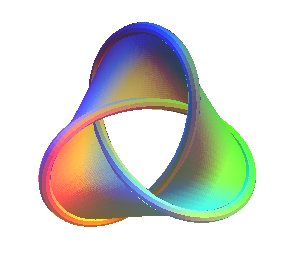
Here are some more properties of Milnor fibers:
- 1.
Each fiber is parallelizable;
- 2.
Each fiber has the homotopy type of a cell complex of dimension .
19 April 9
Paul used GP/Pari to force Zoom to record at a higher resolution.
19.1 More Milnor Fibration
Recall the definition of the Milnor fibration from last time. Then recall that is parallelizable and has homotopy type of an -dimensional cell complex. We give some more properties of the fibration:
- 1.
One can show that are all trivial.
- 2.
Each fiber is diffeomorphic to an open (in the analytic topology) subset of a nonsingular complex hypersurface of the form , where is a nonzero constant.
- 3.
Suppose that is an isolated singularity. Then has the homotopy type of a bouquet of -spheres.
Proof of these claims can be found in Milnor’s book, but they are too long for Paul to give them in class.
The key invariant of an isolated singularity is the Milnor number.
Definition 19.1 (Milnor number).
Let be the ideal generated by the partial derivatives of . Then the Milnor number is simply
Definition 19.2 (Milnor number, second definition).
Let be given by the . This induces a map on a smapp sphere . The degree of the map is the induced map on .
Theorem 19.3.
The Milnor number is the number of spheres in the bouquet attached to the isolated singularity. In particular, .
Example 19.4.
The Milnor number of is . From the explicit drawing of the surface, we can see a homotopy down to a graph with the same homotopy type as .
This is an example of something called a Brieskorn variety, which is a variety of the form . In this case, we can simply compute
Recall that we can consider the monodromy of the fibration. Then this gives an automorphism of , and we can regard as an element of .
Theorem 19.5 (Deligne-Griffiths).
is a unipotent matrix. This means here that is conjugate to an upper triangular matrix with eigenvalues roots of unity. Moreover, all Jordan blocks of have dimension at most .
Example 19.6.
Let . Then we can explicitly compute the eigenvalues of the monodromy map. In fact, they are all products of the form
where is a nontrivial -th root of unity. For example, in the case , the two eigenvalues are the primitive sixth roots of unity.
We will now sketch a proof of the formula. First, we can extend the fibration to all of . We can show that the fiber above is . We can now compute the monodromy of this fibration, which is simply
Then the monodromy is simply . By a result of Pham, we see that the fiber above deformation retracts onto the iterated join of the . For example, the join of is simply the complete bipartite graph .
Example 19.7.
If we label some vertices on the Seifert surface we drew last time, then we can see the graph.
We can now compute the reduced homology of , and we see that the top homology is simply
Remark 19.8.
Results extend to weighted homogeneous polynomials . Here, is weighted homogeneous of tope if it is a linear combination of monomials where
20 April 14
Paul calculated and in GP/Pari.
20.1 Globally Symmetric Spaces
Example 20.1.
Let be the upper half plane and (or some finite-index subgroup), and then we can consider the space . This is a locally symmetric space, which is simply a punctured Riemann surface. There are two obvious compactifications:
- 1.
Fill in the missing points;
- 2.
Fill in the missing points with a bounding circle.
Why is this a locally symmetric space? It is a quotient of a global symmetric space. Here, if and , then .
Definition 20.2.
Let be a Riemannian manifold with an involution for each that fixes but reverses every geodesic through . Then we call a symmetric space. Note that any such is complete because we can extend geodesics by flipping. Also note that has a transitive isometry group.
Example 20.3 (Basic Examples).
- 1.
is always a symmetric space. Here the geodesics are straight lines and the involutions are reflections.
- 2.
Any sphere is a symmetric space.
- 3.
Any hyperbolic space is a symmetric space.
20.1.1 Classification
These spaces were classified by Elie Cartan, which was one of the first major results in the classification of Lie groups and Lie algebras. Here, is a product of three types of symmetric spaces:
- •
Euclidean type ();
- •
Compact type;
- •
Noncompact type;
These are characterized by conditions on their sectional curvature (identically zero, nonnegative, nonpositive).
Next, any symmetric space can be factored into irreducible symmetric spaces. Therefore, we simply need to classify the irreducible symmetric spaces. These were classified using algebra, and are all , where is a connected Lie group and is a maximal compact subgroup.
First, we classify all possible Lie algebras, then see which Lie groups have a given Lie algebra. Finally, using the theory of root systems and weights, we obtain classical families () of symmetric spaces and exceptional examples (). Each one comes in a compact version and a noncompact version. In fact, there is a duality between the compact spaces and noncompact spaces.
20.1.2 Basic Examples
- 1.
Let and . Then and has dimension . The symmetry comes from the involution .
- 2.
Let . Then and has dimension and is called the Siegel upper half-space. This space arises in the study of moduli spaces of abelian varieties. In fact, this is a Hermitian symmetric space, which means is a complex manifold.
- 3.
Let and . Then , which is hyperbolic -space.
- 4.
Now consider . Then and . This example and the previous one arise when studying algebraic groups over number fields. The upper half-plane corresponds to , corresponds to imaginary quadratic fields, and corresponds to the real quadratic fields. Quotients of give Bianchi manifolds, quotients of give Hilbert modular surfaces, and quotients of give modular curves.
20.2 Locally Symmetric Space
Here, we only require involutions that reflect geodesics in neighborhoods of points. However, every locally symmetric space arises as the quotient of a global symmetric space by a discrete subgroup of .
Example 20.4.
We can consider and . Alternatively, we can consider and where is an imaginary quadratic field. If , then we can take , where is a real quadratic field. Here, acts by on the first factor and by on the second factor.
We can understand the geometry of these space by interpreting them as configuration spaces. We will focus on the case where . Our goal is to understand compactifications of the locally symmetric spaces geometrically. Here, points in correspond to lattices in modulo equivalence relations and with some decorations.
21 April 16
Paul computed some values of the Riemann Zeta function.
21.1 Compactifications of the Space of Lattices
Let . Then consider the global symmetric space . note that any coset is a basis of obtained by rotation. Therefore corresponds to the set of volume ordered bases of up to rotation.
Next, consider the locally symmetric space . Here, gives the lattice generated by the rows of , and thus can be identified by the space of lattices in up to rotation and scaling.
Remark 21.1.
Double coset spaces like are ubiquitous in geometry. Any double coset space really corresponds to the set of -orbits on pairs.
Proof.
Let and for two subgroups of . Then consider the diagonal action of by diagonally. Then we can show that -orbits are in bijection with . □
Example 21.2.
Let and be the maximal Borel subgroup. Then is the flag variety, and encodes the relative positions of two flags in . The Bruhat decomposition shows that this is actually a finite set, indexed by the Weyl group .
Example 21.3.
Consider and . Then we can encode as the set of volume ellipsoids in and the points give metrics on . Then the space , which parameterizes ellipsoids of volume up to rotation. By a result of Euler, this is paramaterized by positive real numbers whose product is .
Therefore, we can consider as the set of orbits in . We can consider the space of lattices in the presence of a fixed metric or the space of metrics in the presence of a fixed lattice.
Remarks 21.4.
The space is very close to being a manifold. It has singularities, but they are very mild (in fact just quotient singularities), so the space is an orbifold. The singularities come from lattices with nongeneric symmetry (with symmetry that is more than just ).
- 1.
We can give up and call this space an orbifold, stack, or some other new term, or we can incorporate decorations with the lattices. We will take the second approach later. This corresponds to replacing with a finite index subgroup.
- 2.
This space is not compact. If we scale the -axis up and the -axis down, this sequence of lattices clearly does not converge. In fact, a theorem of Mahler says that a sequence of lattices diverges to infinity if and only if the length of the minimal nonzero vector converges to .
21.1.1 Topology and Geometry for Small
Let . Then this gives lattices in modulo rotation and scaling. We are looking for a fundamental domain for acting on together with an identification on its boundary. This is known as explicit reduction theory.1
First, we will find a shortest nonzero vector . If we rotate and scale onto , we can choose the minimal length vector from the row immediately above the -axis. Then and lies in the strip between and . This gives the famous picture of the fundamental domain in the upper half plane. The two vertical lines are clearly identified, and then the arc the arc is folded in half. Therefore, the space is topologically equivalently to a disc.
22 April 21
Paul computed some values of -functions of number fields in GP/Pari. He then mentioned the class number formula.
Last time, we discussed the space of lattices modulo rotation and scaling. In addition, we computed the fundamental domain of the action of on the upper half-plane.
22.1 Geometry for
We now consider the space of lattices in . We can rescale to make the shortest nonzero vector . Then we can rotate the next shortest vector to lie in the -plane, and we can assume that is in the right half of the fundamental domain of . Finally, we choose a lying above the plane. To do this, consider the quotient of by the plane, and we can choose in the inverse image of the shortest nonzero vector in the quotient lattice.
Remark 22.1.
The image of a lattice in a quotient space is not necessarily a lattice.
Next, we consider where we can arrange to be. We can move along the lattice and move to lie over a polygon determined by . In addition, cannot lie inside the unit hemisphere. Therefore, our configuration has dimension and should have a deformation retract onto a compact space of dimensnio .
First, let’s ignore the noncompact dimensions and focus on the compact part. To see this object, we move to the top of the semicircle and look at the possible polygons. Here, the polygon is the set of points whose distance to the origin is smaller than the distance to any other lattice points. This is called the Dirichlet-Voronoi domain.1 Then this three dimensional space is very complicated, and it is easier to describe a finite version. This is simply a cube with four of the vertices truncated. Note the center of the triangular face is the lattice while the center of a hexagonal face is the lattice.
Exercise 22.2.
Find the three remaining special lattices (names can be found in a crystollagraphy book).
We will not consider the higher-dimensional analogues. The quotients are well-understood up to , but the case is unknown. In , we have the lattice, which makes the geometry of the polytope extremely complicated.2 We have no idea how many faces there are, but we do have a few crude estimates. In addition, our algorithm for finding a nice basis of our lattices fails in dimension greater than . It barely works for , but fails for .
Example 22.3.
Consider the lattice with basis . Note that is a strict subset of . However, if we run our algorithm, we only obtain the lattice, which is not .
Remark 22.4.
Even worse, in high dimensions, there exist lattices such that no basis contains a minimal vector (Conway-Sloane).
22.2 Singularities of the space of lattices
We can eliminate these singularities by introducing extra data. We will call these “marked lattices” and our extra data will kill these automorphisms.
Definition 22.5.
A marking on a lattice is a surjective map such that there exists a finite index sublattice such that is fixed by translation by .
Example 22.6.
We can mark using by reduction mod . Here, .
Remark 22.7.
We can think of markings as coming from coloring data on our lattices.
We can consider “ markings.” Then the space of marked lattices is
where is a finite-index subgroup.
Theorem 22.8.
For , all -marked lattices have the same automorphisms. Therefore, the moduli space of marked lattices is smooth. The analogous procedure for abelian varieties is taking a principal polarization.
23 April 23
23.1 Compactifications of Locally Symmetric Spaces
Example 23.1.
Consider . How do we compactify it? How do we add limit points for rays that go off to infinity? If the lines are parallel, do we want them to have the same limit point? This is one of the reasonable ideas, and we obtain a at infinity.
If we forget about rays and just consider lines, we obtain , with a at infinity. In both these examples, we see that points at infinity can be recorded via equivalence relations on geodesics.
Example 23.2.
Let act on by rotation. Then note that any cone with angle is a fundamental domain. How do we compactify this?
- Method 1:
-
We use what we did for . We can extend the action to the compactification of (say the ) at infinity, and we obtain an honest cone.
- Method 2:
-
We now have distinguished rays. We can attempt to use the -parameter family of parallel rays for each of these. Now we glue these lines onto . We will dictate that the two rays bounding one fundamental domain give lines that intersect at a single point. All rays between the two distinguished rays will converge to that single point. In some sense, this is dual to what we did before and we have a hexagon at infinity.
Why would we consider the second method?
- 1.
We gain information that we lost in the first method.
- 2.
This is what happens when we consider toric varieties.
- 3.
When we consider , we need something more like this method.
Now we will consider the space of lattices up to rotation and scaling. Here, our points have a geometric interpretation, so we can try to leverage this. We have two tools to work with:
- 1.
Geodesics in . We can think of adding limit points for families of geodesics.
- 2.
In configuration spaces and moduli problems, we want the points at infinity to have a geometric meaning.1 For us, this means that lattices should degenerate to something more general. There are other contexts:
- (a)
Consider the moduli space of genus curves . When we go to infinity, we pass to stable nodal curves with several components.
- (b)
Consider the moduli space of abelian varieties. These degenerate to various geometric objects.
- (a)
Now if we consider lattices in , consider the family of lattices , this should converge to the -axis at infinity and the -axis at . The moral of the story is that lattices degenerate to subspaces. This may not seem too complicated for , but it is very complex when .
Remark 23.3.
This approach does use geodesics! We are moving around in the upper half-plane.
Now we consider the space of lattices in . Recall this is isomorphic to a quotient of the Soulé cube times . If we start with the standard basis vectors, we can consider the family
As , we simply obtain the -plane.
For another example, consider
In the limit at infinity, we simply obtain the -axis. We can also see “in between” phenomena. Consider the family
We can see that the -direction collapses faster than the -direction, so if we rescale by , we see that the limit is a flag .
Remark 23.4.
We have seen all possible degeneration types. Now we can attempt to look for more refined degeneration data. We observe that the image of the diagonal matrices in is a maximal flat geodesic submanifolds. Therefore, the points at infinity should be parameterized by flags with some extra data.
If we return to the first example . Recall that we obtain the plane as the limit. However, for , the images of give a lattice in the plane. This gives a point in our space for ! If we change to different (say the basis for the lattice), then we obtain a different lattice in our intermediate stage.
24 April 28
Last time we discussed limits of lattices in . We were able to obtain flags by degenerating lattices. Unfortunately, not every flag can arise as the degeneration of a lattice family.
Example 24.1.
Consider with . Then suppose . Suppose we head down to along a geodesic. If is rational, then we go off to infinity. However, if is irrational, the picture is much more subtle.
- •
If is contained in a real quadratic field, then the path approaches a periodic geodesic.
- •
Otherwise, the path wanders around the quotient and does not escape to infinity. The behavior here is completely unknown.
In terms of flags, only certain flags will arise as limit points, and in fact, we want rational flags. These are flags whose subspaces are generated by lattice points. What about limiting shapes of lattices?
When , we have three types of limiting flags: a plane, a line, and a line inside a plane. When we have a plane, we have a shape inside the limiting plane. In the case of a line, we expect a shape inside the quotient of by the line. Finally, in the case of a full flag, we expect no shape data. More generally, for a flag
we can look at pairwise successive quotients and find lattice shapes there. Putting it all together, we obtain the reductive Borel-Serre compactification. Strata are induced by rational flags in including the empty flag.
For example, we can add three different types of strata when . We can index them by partitions of where the order of the parts matters.
| Flag | Partition | Strata |
|---|---|---|
| -dimensional strata | ||
| -dimensional strata at infinity | ||
| -dimensional strata at infinity | ||
| -dimensional strata at infinity |
In fact, the strata at infinity are lower-rank locally symmetric spaces that are being compactified themselves in this process. The space for looks something like this:
This space is singular. We have attached two-dimensional strata to a five-dimensional space. We can compte links by realizing the space as a quotient of a manifold with corners. The bigger space is called the Borel-Serre compactification.1 There will be a five-dimensional stratum and two four-dimensional strata that meet in a three-dimensional corner. In fact, the four-dimensional strata are fiber bundles over the locally symmetric spaces for .
Consider the case when . Suppose are parallel geodesics that go off to infinity. Should they go to different limiting points or the same point? Recall our discussion about compactifying . There are two answers here:
- 1.
We can send them to the same point because of the metric on the upper half plane. This is because the two geodesics get arbitrarily close together.
- 2.
The geodesics hit different points on various parallel horocycles.2 Thus sending them to different points also makes sense.
To add this data in our lattice/flag description, we add a real transverse flag to the data. The transverse flag corresponds to adding an at infinity. This is really the matrices of the form
In the quotient, this circle is collapsed down to a point.
When , we add flags to the strata corresponding to the compositions . In the Lie groups picture, the three strata correspond to parabolic subgroups. Then the fiber above each point in the two dimensional strata is a torus. Then the three-dimensional stratum is the image of the matrices of the form
and is called a nilmanifold of the Heisenberg manifold.
Exercise 24.2.
Compute the links of points in the strata using the presentation as a space with thin singularities.
Remark 24.3.
It is an open question to generalize these constructions to the nonarchimedean setting. Here, we want to replace real Lie groups with reductive groups over and with the same group over . For example, we replace with and with . The analogue of in this setting is called a building. Compactifications of in this setting have been studied, but locally summetric spaces have not been studied.