Log GLSM and related topics
Abstract.
These are live-TeXed (for all talks besides my own and those of Shuai Guo, some figures were inserted later using Codex or Claude Code) notes from the log GLSM summer school at Sichuan University in July 2026. Note that all talks (besides mine) were given in Chinese. I apologize for any translation errors as well as for any errors in my lectures. In addition, the notes for the two lectures by Shuai Guo are experimental AI-generated transcriptions of his slides. While I did give Claude access to all of my other notes to see what my writing style is, please let me know if there is a mismatch in writing style or if there are any errors. Finally, I would like to thank You-Cheng Chou, Tingting Fang, and Yaoxiong Wen for pointing out mistakes in the notes.
1 Theta-stratifications (Yaoxiong Wen and Bin Wang)
1.1 Our first moduli problems.
Our first moduli space will be , which parameterizes -dimensional linear subspaces in , or equivalently is the geometric quotient . In this case every -orbit in is closed. This construction is our first example of geometric invariant theory. In general, a set-valued moduli problem assigns to every scheme a collection of isomorphism classes of families over , and we can think of it as a functor
Example 1.1.
Let be a smooth projective curve. Then consider the assignment
where and denotes isomorphism of vector bundles on . This parameterizes isomorphism classes of families of vector bundles on , but it is still not the correct stack-valued moduli problem.
Example 1.2.
By the Yoneda Lemma, every scheme defines a moduli problem.
Unfortunately, not every groupoid-valued moduli problem can be represented, as a stack, by a scheme or algebraic space. A scheme or algebraic space has trivial inertia, whereas objects in a moduli problem may have nontrivial automorphisms. For example, if we consider the moduli of line bundles on , each line bundle has an entire of automorphisms. Therefore, when we consider moduli problems, we need to remember both the objects and the isomorphisms between them, and the target of the functor should be the category of groupoids.
Definition 1.3 (informal).
A stack over is a pseudofunctor
which satisfies descent for objects and morphisms with respect to the fppf topology.
Example 1.4.
Consider the stack which sends a scheme to the groupoid whose objects are vector bundles on such that every geometric fiber has rank and degree , and whose morphisms are isomorphisms of vector bundles on .
Unfortunately, there are far too many stacks to consider, so we will need to consider a subclass of stacks which is amenable to the methods of algebraic geometry.
Definition 1.5.
An algebraic stack is a stack with representable (by algebraic spaces) diagonal and with a smooth surjective morphism from a scheme (which is called an atlas).
Note that the first condition means that for any morphism from an algebraic space, then is an algebraic space. This is equivalent to all Isom sheaves being algebraic spaces and implies that any morphism from a scheme to is representable.
Remark 1.6.
For sets, if we have morphisms and , then the fiber product is
For schemes or algebraic spaces, the same formula describes the -points of the scheme-theoretic fiber product. For stacks, a -point of the -fiber product is a triple , where , , and
is an isomorphism in . Thus equality must be replaced by an isomorphism, and the isomorphism must be recorded as part of the data.
1.2 Quotient stacks.
Let be an algebraic group and let be a scheme with a left action of .
Definition 1.7.
The quotient stack sends a scheme to the groupoid whose objects are diagrams
where is a right principal -bundle for the fppf topology and satisfies . A morphism from to is an isomorphism of principal -bundles compatible with the maps to .
Example 1.8.
Let be a smooth separated DM stack of finite type over . If either the generic stabilizer of is trivial or the coarse moduli space of is quasi-projective, then is a global quotient [EHKV01]. Here, a DM stack is an algebraic stack with unramified diagonal, and a global quotient means a stack of the form for some algebraic space with an action of .
Exercise 1.9.
Show that the groupoid is equivalent to the action groupoid of acting on .
After choosing one representative of each -orbit, the above exercise implies that, as an abstract groupoid and not as an algebraic stack, we have
where is the stabilizer of .
1.3 Fine vs coarse vs good moduli spaces.
Definition 1.10.
A fine moduli space for a moduli problem is a scheme or algebraic space which represents the functor.
Unfortunately, it is very hard to find a fine moduli space, so we want to weaken this condition.
Definition 1.11.
A coarse moduli space for an algebraic stack is a morphism to an algebraic space such that
- (1)
For every algebraic space , composition with induces a bijection
- (2)
For every algebraically closed field , the induced map
is a bijection.
Even these do not always exist. A good moduli space is a different weakening: it replaces the requirement of a bijection on geometric points by a cohomological affineness condition [Alp13].
Definition 1.12.
A quasi-compact morphism from an algebraic stack to an algebraic space is a good moduli space if
- (1)
The pushforward functor is exact;
- (2)
The natural map is an isomorphism.
| Notion | Defining property | Geometric behavior | Feature |
|---|---|---|---|
| Fine moduli | Represents the set-valued moduli functor | Its points represent the objects recorded by the functor | Admits a universal family |
| Coarse moduli | Universal for maps to algebraic spaces and bijective on geometric isomorphism classes | One geometric point for each isomorphism class | Forgets automorphisms |
| Good moduli | Cohomologically affine and | May identify distinct nonclosed points | Gives -equivalence in GIT-type examples |
The existence of these moduli spaces is not determined only by whether stabilizers are finite or infinite. For example, is both a coarse moduli space and a good moduli space, even though its stabilizer is .
Theorem 1.13 (Keel-Mori [KM97]).
Let be an algebraic stack of finite type over . If its inertia morphism
is finite, then admits a coarse moduli space. The fiber of over a geometric point is the automorphism group .
Theorem 1.14 (Alper–Hall–Rydh [AHR20]).
Let
be a good moduli space, where is a Noetherian algebraic stack over with affine diagonal. Let be a closed point, and denote its stabilizer group by .
Then there exists an affine scheme equipped with an action of , together with a Cartesian diagram
where
is an étale neighborhood of .
For , the stack is locally of finite type, but it is neither quasi-compact nor separated. To see that it is not quasi-compact, choose line bundles and of degrees and , respectively, and consider
The bundle contains a line subbundle of degree . In any quasi-compact family of vector bundles of fixed rank and degree, the degrees of line subbundles are bounded above, so the bundles cannot all lie in a quasi-compact substack as . To see that the stack is not separated, note that every vector bundle has scalar automorphisms . Stabilizer groups of a separated algebraic stack are proper, whereas is not proper. Passing to semistable bundles does not make the stack separated; rather, it cuts out a bounded open substack of finite type which admits a good moduli space whose closed points are -equivalence classes.
Definition 1.15 (Slope stability).
For a nonzero vector bundle , define its slope by
The vector bundle is semistable if
for every nonzero proper saturated subsheaf , and it is stable if the inequality is strict. Since is a smooth curve, a saturated subsheaf of a vector bundle is a subbundle, so it is equivalent to test nonzero proper subbundles.
Armed with this definition, we may now consider the open substack . Semistable bundles of fixed rank and degree form a bounded family, so this stack is of finite type, and in particular quasi-compact. It is still not separated because every object has the nonproper scalar stabilizer .
Definition 1.16 (S-equivalence).
Let be a semistable vector bundle. A Jordan–Hölder filtration of is a filtration
such that every quotient is stable of slope . The filtration is not necessarily unique, but the associated graded vector bundle
is unique up to noncanonical isomorphism. Two semistable vector bundles and of the same slope are S-equivalent if .
Now we consider the moduli space of -equivalence classes of semistable vector bundles on . There is a good moduli space morphism
and the closed points of are in bijection with -equivalence classes of semistable vector bundles.
Remark 1.17.
The original method of proof for this theorem was to construct the moduli space using geometric invariant theory. The goal of this series of lectures will be to discuss an intrinsic approach using -stratifications together with existence criteria for good moduli spaces, without first choosing a GIT presentation.
1.4 Theta-stratifications.
The framework of -stratifications and numerical invariants used here is developed in [Hal14].
Let be an algebraic stack and consider , where the action on points is ; equivalently, the coordinate function has weight . Assume that the mapping stacks below are algebraic. Then define the stack of filtered objects and the stack of graded objects. There are canonical morphisms
Here is restriction to , is induced by the inclusion , and is induced by the projection . In particular, . We also write .
Definition 1.18.
A -stratum in an algebraic stack is a union of connected components such that the restriction
is a closed immersion.
A -stratification of consists of
- (1)
A totally ordered set with a least element ;
- (2)
An increasing collection of open substacks , indexed by , such that
and such that for every , the set has a least element;
- (3)
For every , a -stratum such that
The semistable locus is , and the stratification gives a disjoint decomposition
Consider the stack . We will consider the stack
Any such map is equivalent to a -equivariant principal -bundle over . When , this is equivalent to a -equivariant vector bundle on , or equivalently to a finitely generated graded locally free -module
With the convention above, the coordinate function has weight , so multiplication by gives maps
Since is locally free over , multiplication by is injective.
Remark 1.19.
Consider the vector bundle . Since acts freely on , equivariant descent gives
where is the projection. Equivalently,
Define
Since , we have . The finite generation and local freeness of imply that this is a finite, exhaustive, and separated decreasing filtration by subbundles, which may be written as
In the other direction, let be a vector bundle with a finite decreasing filtration by subbundles such that the quotients are locally free. The Rees construction is the graded -module
It is locally free over , and its fibers at and satisfy
Therefore, a map from to the stack of vector bundles is equivalent to a finite -weighted filtration of a vector bundle by subbundles with locally free associated graded pieces.
1.5 Non-abelian localization.
We will begin with the classical setting. Let be a smooth projective variety with an action of , let be a -equivariant perfect complex, and write
for the decomposition of the fixed locus into connected components. After localizing the representation ring so that the equivariant Euler classes below become invertible, we have
where
We will now consider the stacky version. Let
be a -stratification. Since is a closed immersion, we may identify with its image in . The center of the stratum is
where is induced by the projection .
Theorem 1.20 (Virtual non-abelian localization [Hal15, Theorem 5.1]).
Let be a quasi-smooth derived stack with a -stratification
where we identify every stratum with its image under , and let be its center. Decompose the restriction of the cotangent complex according to the -weights as
where the homology of , , and is concentrated in negative, zero, and positive weights, respectively. Define
Here and denote the determinant and virtual rank of the perfect complex . We say that a complex of vector spaces is finite-dimensional if the direct sum of all of its cohomology groups is finite-dimensional. Let . Assume that
is finite-dimensional for every and is acyclic for all but finitely many . Then is finite-dimensional if and only if is finite-dimensional, and
Here quasi-smooth means that is perfect of Tor-amplitude contained in .
1.6 Geometric invariant theory.
For geometric invariant theory, see [MFK94]. The vector-bundle example below uses the Harder–Narasimhan filtration [HN74].
Let be a reductive group and be a projective scheme equipped with a -equivariant line bundle . The semistable locus can be defined using the Hilbert-Mumford criterion, where it consists of all points where for all cocharacters , we can define the point
and define the quantity
A point is semistable if for all cocharacters of . The stable locus consists of all points where the inequality is strict and the stabilizer is finite.
Theorem 1.21 ([MFK94]).
The stable and semistable loci are open in . Moreover, is a good quotient and is a geometric quotient.
Example 1.22.
Consider the moduli stack of vector bundles of rank and degree on a curve of genus at least . Then recall that the semistable locus was defined to consist of slope semistable vector bundles. In fact, this can be obtained via GIT.
Fix an ample line bundle on . Then there exists some such that for all and , is globally generated. Therefore, we can consider
If we set , where , then there is a surjection
Therefore, we can think of as a member of a Quot scheme. On the Quot scheme, we can consider the universal family
Now define the line bundle
for some . We can also consider the action of on the Quot scheme. For some cocharacter , we can split
with weights and . Then consider
and consider the filtration
induced by this. Then we see that
Then we compute the restriction and obtain the spaces and , and therefore the weight of is given by
which recovers GIT.
We will now consider the unstable locus. Let be a vector bundle on . Then there exists a unique filtration
such that
- (1)
All are semistable;
- (2)
We have for all .
Remark 1.23.
From the GIT perspective, we should really take to be the reduced Hilbert polynomial.
1.7 Construction of Theta-stratifications.
Let be a reasonable algebraic stack.1 Now consider some family over . If we restrict to the central fiber, we see that acts on , which means we have a map , and from this we can compute the weight.
Note that the morphism is a -contraction, and therefore
Example 1.24.
Let . Then we have
where is the parabolic subgroup corresponding to the cocharacter , and we can always choose representatives in a single Weyl chamber. Moreover, we have
where is the Levi subgroup corresponding to .
Definition 1.25.
A -stratum in is a union of connected components such that
is a closed immersion.
Roughly speaking, closed immersions are injective, so an object in consists of an object in and a “canonical filtration.”
Definition 1.26.
A -stratification is an increasing family of open substacks
where is some totally ordered set, together with -strata
which are required to satisfy
In particular, this implies that
Analogously to the Hilbert-Mumford criterion, we will construct -stratifications using numerical invariants.
Definition 1.27.
A numerical invariant with values in a totally ordered set consists of an assignment of a scaling invariant function
for any and any nondegenerate homomorphism . These are required to satisfy
- (1)
The assignment is invariant under field extensions. This point will not be elaborated on because we are working over ;
- (2)
If we have , then we have a factorization ;
- (3)
If we have some and with finite kernel, the function is locally constant on , where ranges over points of .
We will give a naive version of a construction starting with a numerical invariant . Define to be semistable if for any nondegenerate satisfying . If is unstable, then we define its instability level
If a filtration attains this supremum, we call it a “Harder-Narasimhan filtration.”
Definition 1.28.
A numerical invariant is standard if
- (1)
and are not both positive for ;
- (2)
Each function is strictly quasi-concave, namely for all and linearly independent such that , then
If either value is strictly positive, the inequality is required to be strict.
The next condition is that we need some kind of rationality. We consider , and our goal is to find the rational points. This leads us to condition (R): if attains a positive value for some , then it attains a maximal value at a rational point.
Theorem 1.29 ([Hal14]).
Let be a stack and be a standard numerical invariant satisfying condition (R). Then defines a -stratification if and only if it satisfies the following:
- •
For any DVR with fraction field and residue field , then (HN-specialization);
- •
For any map from a finite type scheme, there exists a quasi-compact open such that for any point of finite type and a filtration of for which , there exists another filtration of with satisfying (HN-boundedness).
The point here is that the conditions of being standard and (R) combined with HN-boundedness imply existence and HN-specialization implies uniqueness.
2 Intro to log geometry (Tingting Fang and Zijian Han)
2.1 Motivation.
In enumerative geometry, we will consider intersection numbers on compactified moduli spaces. This is going to require our objects to degenerate in some way, for example for domain curves to be nodal, maps to land in boundary divisors, or we degenerate the target. In ordinary geometry, we view these as singular, but in log geometry, there is a way to think of these situations as being log smooth. In log geometry, we are going to replace functions with the data of functions and how they vanish on the boundary (or namely the morphism ).
Example 2.1.
Consider a family of curves over , where the central fiber is nodal. In log geometry, if we place the divisorial log structure on , then this family is log smooth.
2.2 Monoids.
Definition 2.2.
A monoid is a commutative semigroup with a unit.
For a monoid , we may associate a group via the standard Grothendieck construction
Definition 2.3.
If the natural morphism is injective, we say that is integral.
Example 2.4.
If has generators with relation , then in we have , so is not integral.
Definition 2.5.
A monoid is
- •
fine if is finitely generated and integral;
- •
saturated if for all and all natural numbers , if then ;
- •
torsion-free if is;
- •
sharp if the identity is the only invertible element.
2.3 Log structures.
Let be a scheme.
Definition 2.6.
A pre-log structure on is a sheaf of monoids on the small étale site of and a morphism . It is a log structure if , where the isomorphism is given by .
We now consider the exact sequence
and the quotient here is called the characteristic sheaf or the ghost sheaf.
Example 2.7.
Let and be the identity. Then there is no additional information provided by the log structure.
Example 2.8.
Let be a regular variety and be a closed subscheme. Set . Then define
where is the open immersion. If is a divisor, then this is called the divisorial log structure.
For example, if and , then the characteristic sheaf vanishes everywhere except for the origin. Here, we compute
The stalk is everywhere except at the origin, where it is .
Example 2.9.
Now let and be the union of the coordinate axes. Then
Note here that at the general point, we see . At the origin, we see . At a general point on the -axis, we see that is invertible, so we see the stalk . Similarly, we can compute the stalk at a general point on the -axis.
Just as we can associate a sheaf to a presheaf, we will associate a log structure to a pre-log structure. First, a pushout in a category will be denoted by and is the colimit of the diagram
In the case where is commutative monoids, then
Example 2.10.
Consider the morphisms and . Then the pushout is the monoid
If we replace by the category of sheaves of commutative monoids, we can form the pushout on sections and then sheafify.
Definition 2.11.
The associated log structure of a pre-log structure is the pushout
The map to is given by .
Definition 2.12.
A morphism of log schemes consists of
- (1)
A morphism of underlying schemes;
- (2)
A map , where is the log structure associated to .
Definition 2.13.
A chart for a log scheme is a morphism from the constant monoid such that , where .
Charts are useful in specifying log structures. For example, if we have , then gives a log structure on .
Example 2.14.
The trivial log structure is given by the chart .
Example 2.15.
Let and give a log structure by which sends to and to . This is called the standard log point and can also be formed by restricting the divisorial log structure on to the origin.
Example 2.16.
Consider the chart which sends . Then this recovers the divisorial log structure on relative to the origin.
Example 2.17.
Consider the chart which sends . This recovers the divisorial log structure on relative to the toric boundary.
Definition 2.18.
A chart for a log map is a triple , where and are charts and the diagram
commutes.
Definition 2.19.
A log scheme is finitely generated, fine, integral, saturated if there exists an étale local chart for a cover such that is finitely generated, fine, integral, or saturated, respectively.
2.4 Log smoothness.
Definition 2.20.
Consider a commutative diagram
where is a strict closed immersion (here, this means that ). A morphism of fine log schemes is log smooth (resp. log étale) if
- (1)
The underlying map is locally of finite presentation;
- (2)
For any commutative diagram as above, étale locally on there exists a (resp. there exists a unique) morphism such that and .
We will now give a chart local criterion for log smoothness.
Theorem 2.21 ([Kat89, Theorem 3.5]).
Let be a morphism of fine log schemes. Assume we have a chart where is a fine monoid. Then is log smooth if and only if étale locally on there exists a chart for extending satisfying
- (1)
The kernel and the torsion part of the cokernel of are finite groups whose orders are invertible on ;
- (2)
The induced morphism is étale in the classical sense.
Example 2.22.
Let be an affine toric variety given by for a monoid . Note that induces the divisorial log structure. Then consider the map , where the point has a trivial log structure. We note that the morphism has no kernel and the cokernel is torsion-free, and the map
is an isomorphism, so any toric variety is log smooth over a point with trivial log structure.
From this example, we can morally think of log smoothness as being locally toric relative to the base.
Example 2.23.
Recall the family with log structure relative to the central fiber over with the divisorial log structure relative to . The map of charts we will consider is in fact . Taking the groupification, the map becomes . The kernel is trivial and the cokernel is torsion-free, so we have verified the first condition. Then we consider the map
which is an isomorphism, so this family is log smooth.
2.5 Stack of log structures.
The stack of log structures and its relation to log smoothness are due to Olsson [Ols03].
Let be a fine log scheme. We will consider the category whose objects are fine log schemes and whose morphisms are strict morphisms over .
- (1)
This category is a category fibered in groupoids over classifying all fine log schemes mapping to ;
- (2)
is an algebraic stack locally of finite type over ;
- (3)
A morphism is log smooth if and only if is smooth. The same holds with smooth replaced by étale.
2.6 Tropicalization.
Let be a fine log scheme. Then the tropicalization of is defined to be the colimit
where the equivalence relation is given by if a point specializes to , then the induced map induces an equivalence from to its image.
Now suppose there is a stratification of by such that is constant. For any , all points satisfy , so we only need to consider the generic points of the strata and then glue various faces.
Example 2.24.
Consider with the trivial log structure. Note that for any point , we have , so . Then .
Example 2.25.
Consider relative to the origin (with divisorial log structure). It is easy to see that and , so the tropicalization is .
Example 2.26.
Consider with the toric log structure (divisorial log structure relative to ). Then , , , and , so we obtain the fan of as a toric variety treated as a cone complex.
Example 2.27.
Let be a toric variety with the divisorial log structure relative to . Then
so a possible slogan is that tropicalizing a toric variety recovers the structure of ordinary toric geometry (minus the embedding of the fan in some real vector space).
Example 2.28.
Let with divisorial log structure over . Then there is a chart given by
Note that and . Therefore, we have
at the singular point , which recovers the cone which gives as a toric variety. At the generic point of , we see that , and therefore . Similarly, we see that . The remaining problem is gluing.
Note that is given by , , and , and therefore the map sends to , where .
The morphism giving a family of curves with nodal central fiber has tropicalization given by projecting the cone onto .
2.7 Log curves.
For now, all monoids and log schemes will be fine (or even fine saturated). There are two reasons for this:
- (1)
If is a fine monoid, its dual is fs and sharp;
- (2)
If is a fine log scheme, for any geometric point , there exists an étale neighborhood of which has a chart.
We will now discuss various geometric properties of maps between monoids.
Definition 2.29.
A map is integral if the map is flat.
For example, any nonzero map and the diagonal are integral. If a map is integral, then for any , the monoid is fine.
Example 2.30.
Pushouts may not be fine, for example consider
Definition 2.31.
A map between fine log schemes is integral if at every geometric point of , the map
is integral.
Definition 2.32.
A map between fs monoids is saturated if for all , the monoid is also fs.
Example 2.33.
The map is saturated, but is not.
Definition 2.34.
A log curve over an fs log scheme is a log smooth and integral map between fs log schemes such that the underlying geometric fibers are reduced connected curves.
Proposition 2.35 ([Kat89]).
Let be a log smooth and integral map between fs log schemes. Then is flat.
Theorem 2.36 ([Kat00]).
The underlying family of a log curve is a family of nodal curves.
Example 2.37.
Let . Then is log smooth over , but is a cusp.
Definition 2.38.
An -pointed log curve over an fs base consists of the data such that
- (1)
The underlying family is a prestable curve;
- (2)
is a log smooth map between fs log schemes;
- (3)
On the smooth locus of , we have
2.8 Canonical log structures on prestable curves.
Let be the moduli of -pointed prestable curves. Then the singular locus is a normal crossings divisor, so there is a canonical log structure
If we consider the universal family , we can form . Therefore, we have a map
We can also consider the divisors , which also define log structures
Therefore, we can define a log structure
Then if we consider
we can lift to a map of log stacks.
Theorem 2.39 ([Kat00]).
The map is a log smooth integral map.
Definition 2.40.
For a family of prestable curves, we can pull back along the diagram
and endow the left edge with a canonical log structure.
Remark 2.41.
Let . If , then is the number of nodes on . Working étale locally on a node , the log structure looks like
Theorem 2.42 ([Kat00]).
Let be an -pointed log curve on an fs base . Then there exists a unique such that
is a Cartesian diagram in the category of fs log schemes.
A slogan is that a log curve is a prestable curve together with .
Example 2.43.
Let and . Also choose . Then consider the diagram
On log structures, consider the case where the bottom left arrow corresponds to on . Then at the top left corner, the monoid becomes . If we call this , then the map is not a family of log curves with the canonical log structure, but is a family of log curves.
2.9 Moduli of log curves.
Definition 2.44.
A map between -pointed log curves is a pair such that is strict and the diagram
is Cartesian. Denote by the fibered category parameterizing -pointed log curves.
In particular, for a scheme , the groupoid parameterizes log structures together with log curves .
Consider a log curve over . Denote . At a generic point or a general smooth point , the map is
At a marked point , we have . In this case we have
the specialization map and the pullback
At a node , we have . Let denote the image of in , which is the edge length or smoothing parameter at . Denote by and the generic points of the two branches of . Then the generalization maps are
2.10 Tropicalization of log curves.
We will only consider the situation over a log point . We will consider the category of cones , whose objects are pairs such that , where is a full-dimensional strongly convex rational polyhedral cone. The morphisms are maps , which consist of
such that .
Example 2.46.
Let be an fs log scheme and consider .
We will now consider the category of generalized cone complexes. Its objects are topological spaces together with a presentation as the colimit of a diagram in with all arrows being inclusions of faces. Its morphisms are continuous map such that for each , the map factors through .
Example 2.47.
If is a morphism of fs log schemes, the map induces on tropicalizations.
Definition 2.48.
A cone complex is a generalized cone complex such that for each , the map is injective.
Theorem 2.49 ([ACP15]).
If is fs and log smooth over with Zariski log structure, then is a cone complex.
For a monoid , we will denote and the lattice . At a smooth point, we have
At a marked point, we see that
At a node, we have
Note that the cone is in fact equal to
Now that we understand the cones associated to every point, we now need to discuss the face maps. The generalization maps corresponding to marked points are
and the associated face maps are
At a node, the two face maps are
and
Example 2.50.
Consider a curve which is a union of two rational curves with a marked point on one branch. Then let . Then we see that
, and . We also see that and .
2.11 Tropical curves.
Definition 2.51.
A family of tropical curves over a cone consists of
- (1)
A connected graph ;
- (2)
A leg ordering ;
- (3)
A genus function ;
- (4)
An edge length function .
Now we will construct . For , we set . For , we set
For legs , we set . We now need to define the face maps. If is incident to , then the face map is
If is incident to two vertices , then the face maps are
Remark 2.52.
The choice of and does not change the cone complex up to isomorphism, but it does matter when we want to define contact orders for log maps. However, in general there is no canonical way to make this choice.
2.12 Punctured curves.
Punctured logarithmic curves and maps are developed in [ACGS25].
We consider a nodal curve
with log structures given by with chart and being the standard log point. Now consider and mark the node by . Note that
Denote . Then we see that on log structures we have the diagram
In particular, we can compute the stalk , and therefore we have
However, we should have the map
and therefore is not a log curve. We can then consider the diagram
Therefore, we will consider extending the log structures.
Recall that for a log curve, we have , where is the divisorial log structure by the markings.
Definition 2.53.
A punctured curve over an fs log scheme consists of , where is a log curve and the map is a map of fine log schemes satisfying the following conditions:
- (1)
The underlying map is an isomorphism;
- (2)
On log structures, the map is an isomorphism away from the and induces
- (3)
For any marking and any , we have .
Roughly speaking, a punctured curve is a log curve plus the data of a commutative diagram
Example 2.54.
Let be a smooth -pointed curve.
- (1)
Let be endowed with the canonical log structure (so has no log structure). Let . Then any puncturing must be trivial. The reason is that cannot have a section such that . If , then . Otherwise, if , then because is nonzero, so is .
- (2)
Let be a puncturing. Choose a local generator of . Then any has the form where and . If , then we require that . This implies that , and therefore
In fact, any fine submonoid of the right hand side containing can be realized by a puncturing.
- (3)
Let . Consider such that . Because , we see that is not saturated.
Lemma 2.55 ([ACGS25]).
Let be a sharp fs monoid. Let . Let be finitely generated with and . Then there exists a nonzero, concave, piecewise linear function
with rational slopes such that
Example 2.56.
Let and set
Then
3 Intro to GW theory with a view to higher genus (Patrick Lei)
3.1 Introduction to GW theory.
For the virtual fundamental class construction, see [BF97]; for the axioms and quantum cohomology, see [KM94].
The goal of these lectures is to discuss Gromov-Witten theory in a way that is amenable to doing calculations in higher genus. Gromov-Witten theory concerns itself with integrals on the moduli space , where is a smooth projective algebraic variety and is an effective curve class. There is a diagram
where is the universal curve, are the sections of which give the marked points, is the universal stable map, and are evaluation morphisms. While is generally singular, not equidimensional, and reducible, there is a special class
which is known as the virtual fundamental class.
Exercise 3.1.
Use standard arguments in deformation theory to verify that the “expected dimension” of is the number given above.
Under the assumption that is smooth and projective, is proper, so we may define GW invariants
for . Here, the are defined by .
Unfortunately, calculating individual Gromov-Witten invariants is very difficult, so we will consider the even more difficult problem of studying generating series of GW invariants, for example
when is a Calabi-Yau threefold. Here, is a formal variable which keeps track of the curve class and we will denote the ring by . There are some other structures we will consider. First, we may consider the quantum cohomology ring, whose product is given by the formula
Here . We will also consider the quantum connection. Let be a basis for . Then the quantum connection is the connection on the trivial bundle with fiber over given by the formula
Sometimes, it is useful to also consider the connection in the -direction given by
where is the grading operator and
is the Euler vector field. Because we will be mostly interested in Calabi-Yau varieties, we will not consider this.
3.2 Enumerative mirror symmetry in genus zero.
The impetus for mathematicians to develop and study Gromov-Witten theory came in the early 1990s, when Candelas, de la Ossa, Green, and Parkes [COGP91] predicted the number of rational curves of low degree on a general quintic threefold by converting the problem to one of computing period integrals on a different Calabi-Yau threefold called the mirror quintic (equivalently, studying its variation of Hodge structure). In genus zero, all invariants can be recovered from the J-function , which is defined by
for any and , where is the Poincaré pairing. Therefore, the problem of computing all genus-zero Gromov-Witten invariants with descendants (these are the -classes) reduces to the problem of computing the J-function.
Remark 3.2.
We expand as .
We should note that the J-function can be obtained via a fundamental solution to the quantum differential equation, which is given by
This has the property that , which is usually known as the symplectic property. From this, we can recover the J-function by .
In physics, mirror symmetry is a duality between two different theories called the A-model and B-model, so now we will need to introduce the B-model object. In the interest of time (and notation), we will assume that is a toric variety and that is nef. Let be the complete set of torus-invariant divisors in . Then define the -function
Note here that we expand any which appears as , or namely, as a geometric series in . In addition, the I-function is annihilated by a differential equation known as the Picard-Fuchs equation, which is some hypergeometric type equation.
Example 3.3.
If and , we obtain
so in fact we see the Bessel function of the first kind as the leading term.
If is a complete intersection in a toric variety cut out by line bundles , all of which satisfy for any genus zero stable map to (this is called being convex), then the quantum Lefschetz theorem [CG07] allows us to replace with and perform all computations on . In this case, the I-function is defined to be
where we abuse notation and conflate the with their first Chern classes.
Example 3.4.
For the quintic threefold, which is cut out by a section of , the I-function at is given by
The content of the genus zero mirror theorem is a correspondence between these two objects. More precisely, in the case where is nef, they are related by a change of variables.
Example 3.6.
When , note that and , so in fact, we have the equality
Example 3.7.
When is the quintic threefold, we will rewrite the components of the I-function as for convenience. We have
so there is a nontrivial mirror map in this case. Specializing to , we see that , so we obtain
By the divisor equation, the left hand side also equals , and we will also refer to this as the mirror map. Therefore, we can use the mirror theorem to compute . The quantum connection in the direction of becomes the ODE
where (here, the coordinate is ) and . An explicit computation using the mirror theorem and the results of Zagier–Zinger [ZZ08] yields
Because begins with the identity, this computes .
3.2.1 Oscillating integrals.
We will now reinterpret the genus zero mirror theorem, and we will return to this interpretation when we discuss higher genus invariants. In particular, we will interpret the I-function as an integral on some mirror family to , which for us will be a toric variety. Let
be the fan sequence of . Applying , we obtain the exact sequence
Suppose that the map is given by the matrix . Then we consider the variety
which is mirror to and consider the superpotential . If we wish to consider the equivariant theory with equivariant parameters acting on each homogeneous coordinate of , we will consider .
Example 3.8.
When , the mirror to is the superpotential on the variety .
We now choose an appropriate Lefschetz thimble near each critical point of the (equivariant) superpotential and consider the integral
This corresponds in the I-function to replacing each in the expression by (turning on the equivariant parameters) and in the J-function to considering the fully equivariant GW theory of . In genus zero, the limit as exists, so we can safely recover the original mirror theorem from the following:
Theorem 3.9 ([Giv96]).
This integral is annihilated by the same Picard-Fuchs equation as the I-function, and up to various prefactors, its asymptotic expansion as along the negative real axis coincides with the restriction of the I-function corresponding to the T-fixed point on which corresponds to the critical point .
3.2.2 The Lagrangian cone.
The quantum cohomology of is an example of a Frobenius manifold, which we will see later can be produced from any cohomological field theory. Write and let be a basis for , so we can write . The structure of a Frobenius manifold comes from the function
which is also called the genus zero descendant potential of . It satisfies the string equation, dilaton equation, and topological recursion relations:
To state the following result, we consider the infinite-dimensional vector space (or a completion of this) with the symplectic form
We also consider the new variable2 , so is now a function near .
Theorem 3.10 (Givental [Giv04]).
satisfies the above PDEs if and only if the graph of is a Lagrangian cone with vertex at such that its tangent spaces are tangent to exactly along .
We may recover the Lagrangian cone by the following procedure. We find a fundamental solution
to the quantum connection, which satisfies the equation
Then, setting , we can then recover the Lagrangian cone by the following procedure:
- •
The derivatives form a basis of ;
- •
This implies that . Writing these in terms of the first derivatives and using the fact that solves the quantum connection, we recover the Frobenius structure and hence the Lagrangian cone.
Using this, we can interpret the genus zero mirror theorem as:
Theorem 3.11 ([Giv98]).
The I-function lies on the Lagrangian cone of .
3.3 Moduli of curves and CohFTs.
The notion of a cohomological field theory was introduced by Kontsevich–Manin [KM94].
We will denote by the moduli space of stable curves of genus with marked points. This is nonempty if and only if , in which case it is a Deligne-Mumford stack of dimension . There is a combinatorial structure to the collection of , which is given by a collection of morphisms.
- •
There is the gluing morphism
which takes two curves and glues them along the last marked point to form a node;
- •
There is the self-gluing morphism
which glues the last two marked points.
There is of course another interesting map, which is the forgetful map
given by deleting the last marked point and then stabilizing. We are now able to define our enumerative theories of interest, which include Gromov-Witten theory.
Definition 3.12.
Given a vector space with a nondegenerate symmetric bilinear form and a unit element , a Cohomological Field Theory (CohFT) on is a collection of -equivariant linear maps
which satisfy the basic identity
and the following combinatorial identities (we will let be a basis of such that and be the dual basis):
If in addition the identity
is satisfied, then we say the CohFT has a flat unit (or satisfies the string equation).
All of this can be generalized to super vector spaces, but for simplicity we will not deal with this case.
Example 3.13.
The most important example of a CohFT is the Gromov-Witten theory of a smooth projective variety . Here, recall that the source of a stable map is a prestable curve, so there is a stabilization morphism
which forgets the map and stabilizes the curve. Then, working over the Novikov ring, we will set , to be the Poincaré pairing, and to be the fundamental class of . The linear maps are given by the formulae
where is the -th evaluation map.
Example 3.14.
Let be the universal curve. Then the Hodge bundle is the vector bundle
We then consider the vector space with the usual pairing and define the CohFT by the formula
The gluing axioms are satisfied by the equation and the exact sequence
Here, because genus zero components do not contribute to global sections of and does not depend on the marked points, this CohFT has a flat unit.
Remark 3.15.
We will see later that this is related to the GW CohFT of a point by the quantum Riemann-Roch theorem.
Given a CohFT , we may produce invariants by pairing the classes with various cohomology classes on . The most important ones to consider are the classes
where is the -th marked point.
Remark 3.16.
In Gromov-Witten theory, these are called ancestors. There are also descendants, which are given by the same formula except using the moduli space of prestable curves instead of , where we factor the morphism defined above as
The descendant classes are denoted by .
Example 3.17.
We will calculate an invariant which will appear in the GW theory of Calabi-Yau threefolds. For any CohFT , consider the invariant
Using the second gluing equation, the degree zero part of is equal to
which yields the (graded) dimension of (for example, if for a Calabi-Yau threefold , this is the topological Euler characteristic of ). Therefore, we obtain
Example 3.18.
Consider the GW CohFT of a point. This is given by with the usual pairing and the formula
Then we define the invariants
Theorem 3.19 (Kontsevich [Kon92]).
The function
is annihilated by the operators
Remark 3.20.
This result (Virasoro constraints for a point) is equivalent to being a tau-function for the KdV hierarchy and has been generalized by various authors.
3.4 -matrix action.
In the early 2000s, Givental discovered a remarkable property of axiomatic enumerative theories, namely that one can transform CohFTs by the action of matrices which satisfy the property
Traditionally, the literature requires that and , but the MSP group has removed this restriction and also allows .
In order to define the action of on a CohFT defined on , we need to review some of the combinatorial structure of . For a curve , we may consider the dual graph of , which has vertices, edges, and legs, which are defined as follows:
- •
The vertices correspond to irreducible components of and are labelled by a non-negative integer, which is the genus;
- •
The edges correspond to nodes of (in particular, we allow loops);
- •
The legs correspond to marked points.
Any graph which appears as the dual graph of a stable curve is called a stable graph.
The first type of action on CohFTs is a translation action. Let . For a CohFT , we define
whenever the infinite sum makes sense.
Example 3.21.
If is the GW CohFT of a smooth projective variety and is a divisor class, then the infinite sum makes sense and we can define the shifted GW CohFT of . For example, if is the quintic threefold and , then shifting to is the same as the mirror map .
The second type of action is the action of a matrix as in the beginning of this section. Let denote the set of all stable graphs of genus with legs. Then we define
where is defined by the following construction:
- •
At the -th leg, we place the map
- •
At every edge, we place the bivector
- •
At every vertex, we place the linear map
- •
Finally, we consider the pushforward in cohomology along the gluing morphism .
Definition 3.22.
Let be as above. Then we define the translation
Whenever it makes sense, we define
Theorem 3.23 (Chang-Guo-Li [CGL26, Theorem 2.7]).
Suppose we work with coefficients in . Then if
is a well-defined CohFT. Moreover, if , is a unit for .
We would like to remark a bit more about the translation action when . For simplicity, we will assume that and for some constant . Then we set and use the dilaton equation to compute
whenever this makes sense.
3.5 Reconstruction theorem.
Recall that every CohFT defines a Frobenius algebra. We will call a CohFT semisimple if the corresponding Frobenius algebra is semisimple.
Theorem 3.24 (Teleman [Tel12]).
Let be a semisimple CohFT with flat unit and be its topological part. Then there exists a unique
such that
Example 3.25.
Recall the Hodge bundle CohFT from before. Recall that it is given by the formula
Taking the degree zero part, we see that is the GW CohFT of a point. Using Mumford’s computation
where , are the Bernoulli numbers, and is the inclusion of the boundary up to a étale cover, and the formula
for any vector bundle (or by just using the quantum Riemann-Roch theorem3 directly), we obtain the -matrix
As a sanity check, we will compute using the -matrix. First, we consider the stable graphs in Figure 2.
The first graph gives us the contribution
Using the formula and the fact that , this becomes
The second graph does not receive tail contributions because . The constant term of the edge contribution is , so considering the automorphism and pushing forward to gives us
where denotes the boundary divisor (with the correct stack structure). Because in this case, we obtain
3.6 Operator formalism and geometric quantization.
We will return to the symplectic formalism of Givental. This is more convenient for certain computations, but it is in fact equal to what we have before, at least when we want to calculate generating functions. Recall that we had a Frobenius manifold structure on and we considered the vector space with symplectic form
If we consider the polarization given by and , then letting be as before (with the dilaton shift), let be coordinates on such that form a system of Darboux coordinates for .
Definition 3.26.
We will call any formal function of the form
an asymptotic element of the Fock space.
Then given such an asymptotic element of the Fock space, we will quantize (infinitesimal) symplectic transformations on by the following formulae:
In particular, this will allow us to understand expressions like . However, we need to be careful because our formulae will involve both the fundamental solution and the -matrix, and is a power series in .4
Theorem 3.27 (Givental [Giv01a]).
An operator of the form acts on (asymptotic) elements of the Fock space by the formula
where is defined by the formula
Operators of the form act by the formula
where is defined by
For a semisimple CohFT, there is a system of canonical coordinates such that the -form is a homomorphism of algebras . Then near a semisimple point, there is an asymptotic solution to the quantum connection of the form
where switches from flat coordinates to canonical coordinates and is the matrix of canonical coordinates. Finally, define
A corollary of Teleman’s reconstruction theorem is the formula
for the Gromov-Witten theory of any smooth projective variety with semisimple quantum cohomology.
Example 3.28.
As a final example, we will apply Teleman’s theorem to compute of any semisimple CohFT. Let denote an idempotent basis for the quantum product. We will compute
Using the reconstruction theorem, we obtain
Using the identities
where , we obtain the result
which can be placed in the suggestive form
This recovers a result which was already known to Givental.
3.7 How to compute the R-matrix.
We will conclude by explaining how to compute the R-matrix, starting in the setting where the Frobenius manifold is conformal (for example the Gromov-Witten theory of a smooth projective variety, -spin curves, etc). In this example, we will consider the Frobenius manifold for 3-spin curves, following [PPZ15]. Let be 2-dimensional with coordinates and , where corresponds to the unit. The metric is given by
and the primary genus zero potential is . There is an Euler vector field
which acts with weights and on and , respectively. The conformal dimension is , and we will define the degree operator
Here, has degree and has degree .
To make our lives easier, we will set and define
and then compute in this frame. In this setting, quantum multiplication is given by
The last thing we need is that quantum multiplication by is given by
We will now compute the R-matrix by using the recursive equation
Setting , we obtain the equation
The unique solution of this is in fact
If you are familiar with tautological relations on the moduli space of curves, you will see that the series and enter in the formulation of the Faber-Zagier relations and the formulation of Pixton’s relations.
In the case where the Frobenius manifold is not conformal (for example in equivariant Gromov-Witten theory), we will need to use an oscillating integral or some other technique to fix initial values in the R-matrix. We will give an example computation here, which is due to Givental [Giv01b]. In this setting, , but the argument can be made to work for any Fano toric variety. Recall that the equivariant mirror of is the superpotential
(here, we change the sign of the equivariant parameters for convenience). Therefore, the oscillating integrals will look like
This is annihilated by the operator
which is exactly the Picard-Fuchs equation satisfied by the I-function of projective space.
To expand this integral near the critical points, we first need to compute the critical points. Here, using coordinates and , we obtain the equation
where is the Lagrange multiplier. These satisfy the equation
and therefore for generic values of , near , the possible values of the Lagrange multiplier are distinguished by which of the they begin with. Note that the function , the values of the Lagrange multipliers, and therefore the critical points, all depend continuously on , so they admit non-equivariant limits at when .
When , the matrix transitions from the flat basis to the basis
which are the leading terms of the canonical coordinates (simply compute the fixed points of the torus action via equivariant localization, and we will obtain this Lagrange interpolation). Therefore, we need to compute in the limit. A direct computation shows that applying to the integral introduces an additional factor proportional to to the integrand of the oscillating integral. Because we can permute the indices, we will compute only the case where . Another direct computation shows that the integral vanishes at unless , so in fact we see that is diagonal in the classical limit. When , we have
and the integral becomes
which is simply a product of gamma functions.
Lemma 3.29.
We have the asymptotics
Using this, we see that at , the diagonal matrix element of the R-matrix is given by
By a result of Givental, this implies that this R-matrix recovers the equivariant GW theory of , and as a corollary, because the non-equivariant limit exists, we obtain Virasoro constraints for .
4 Decomposition theorem for semi-small maps (Xueqing Wen)
Question 4.1.
Let be a (manifold, variety, analytic space, etc). How can we compute ?
Unfortunately, this question is too hard, so we will replace it with a new question.
Question 4.2.
How can we detect using smaller spaces?
Theorem 4.3 (Künneth formula).
We have .
Unfortunately, most spaces are not products, so we consider the following question.
Question 4.4.
Let be a morphism. Can we detect the cohomology of using the cohomology of and the cohomology of the fibers of ?
This question is still very difficult, but at least we can study it. We will begin with the case where is a fiber bundle between compact manifolds. The answer is of course the Leray or Serre spectral sequences, but before we get there, we need some preliminaries.
Definition 4.5.
A -local system on is a locally constant sheaf of vector spaces on .
For example, if is connected, then local systems correspond to representations of . Also, note that if is an algebraic variety, we will need to work with its analytification.
Example 4.6.
Let be a fiber bundle with fiber as above. Then is a local system on with fiber .
Proposition 4.7.
We have
Theorem 4.8 (Leray/Serre spectral sequence).
We have a spectral sequence
We will now consider the setting where is a smooth projective map between smooth projective varieties.
Theorem 4.9 (Deligne [Del68]).
We have the non-canonical isomorphism
At the level of cohomology, we have
This is a consequence of the hard Lefschetz theorem for projective varieties and also states that the Serre spectral sequence degenerates at the page. In topology, this fails for the Hopf fibration.
We will now consider the setting where is a proper map between algebraic varieties. Then we have a Whitney stratification5 such that is a fibration in possibly singular varieties.
Definition 4.10.
A -module on is called a constructible sheaf if there exists a Whitney stratification such that is a local system for all .
With this definition, we may consider the derived category of constructible sheaves on . This assignment admits a six functor formalism, where the functors are , and satisfies Verdier duality via the functor
Definition 4.11.
A complex is a perverse sheaf if it satisfies the following conditions:
- (1)
(Support condition) We have for all ;
- (2)
(cosupport condition) We have for all .
Remarks 4.12.
- (1)
Perverse sheaves are not sheaves, but are complexes in degrees .
- (2)
They have two origins. One is intersection homology, and the other is the Riemann-Hilbert correspondence.
We will need to use the following fact: the category of perverse sheaves on is an abelian category and is moreover the heart of a -structure on . In particular, for any , we can consider the perverse cohomology .
Theorem 4.13 (Beilinson-Bernstein-Deligne-Gabber [BBD82]).
Let be a proper morphism between algebraic varieties. Assume that is smooth and connected.6 Then
Moreover, each is semi-simple (meaning each subobject is a direct summand).
Definition 4.14.
Let be a proper surjective morphism with smooth and irreducible. Let be a stratification such that is a -fibration. We say that is semi-small if for all , we have . If equality holds, we say that is relevant. If the only relevant stratum is the dense one, then we say that is small.
Theorem 4.15 ([CM02]).
If is semi-small, then is a perverse sheaf on .
Proof.
For , we see that
Note that this vanishes if . If we vary over all strata , we obtain the support condition. Because is proper, we have , and by using , we obtain the cosupport condition. □
Examples 4.16.
We now give some examples of semi-small maps.
- (1)
Any generically finite proper map between surfaces is semi-small.
- (2)
Let . Then there is a crepant resolution of singularities, and the fiber over the singular point is a chain of s, so it is semi-small (see also the previous example).
Theorem 4.17 (Kaledin [Kal06]).
A projective birational map from a nonsingular holomorphic symplectic variety is semi-small.
Example 4.18.
For example, the Springer resolution and the Grothendieck-Springer resolution are semi-small. In addition, the Hilbert-Chow morphism for the Hilbert scheme of points on a surface is semi-small.
Let be semi-small and consider a stratification . If is relevant, consider
where . Then is semi-simple. Here, note that . Now let be the intermediate extension of on , which is a perverse sheaf.
Theorem 4.19 ([CM02]).
Let be semi-small. Then there is a canonical decomposition
Example 4.20.
Let be a reductive group with Lie algebra and choose a Borel . Then
is small. Therefore, we have
Recall that is a -torsor. Then for , we have , and therefore . This implies that acts on , and this action can be extended to and also on , and in particular acts on the fiber for any .
Example 4.21.
Consider the Springer resolution . This map is semi-small, but unfortunately all nilpotent orbits are relevant. Note that the fiber above the orbit is a union of two s glued at a node, the fiber above the orbit is a point, and the fiber above the orbit is .
We see that must be trivial because is an isomorphism above this orbit. Then is a rank local system on . Finally, is a rank local system on . Therefore, we have
Restricting to , we obtain . Restricting to , we obtain
Restricting to , we obtain
As representations of , these correspond to the trivial representation, two copies of the standard representation, and the sign representation. For the Springer-theoretic construction and these decompositions, see [BM83].
5 Quantum K-theory (Xiaohan Yan and You-Cheng Chou)
5.1 Overview.
Gromov-Witten invariants are some way of “counting” curves in a smooth projective variety . GW theory produces numbers of the form
for various classes , genus , number of marked points, and curve class . This has been used to study mirror symmetry, and outside of mirror symmetry has produced birational invariants. Our goal now is to lift this entire story to K-theory. Quantum K-theory produces numbers
for . These satisfy various difference equations7 and have found various applications in 3D mirror symmetry and representation theory.
5.2 K-theory.
Definition 5.1.
Let be a smooth projective variety. Then the K-theory of is the Grothendieck group of vector bundles on with the relation that if
is a short exact sequence, then .
Remark 5.2.
- (1)
is a ring with the operations of direct sum and tensor product;
- (2)
The Chern character gives an isomorphism , at least working over .
Example 5.3.
Let and set . Then we have
For a Deligne-Mumford stack which is not assumed to be smooth, then there are two versions
where means coherent sheaves and means perfect complexes. These coincide on a smooth projective variety, so from now on will mean . There is a tensor product
and a pushforward
along proper morphisms. If is a perfect morphism (for example flat, regular embedding, etc), then there is a pullback
5.3 Moduli of curves.
Recall the moduli space
of stable maps to . This has evaluation maps
There are also the universal cotangent lines .
The moduli space is a proper DM stack which has a perfect obstruction theory, which produces a virtual structure sheaf . This comes from the structure of a virtual tangent bundle, where
Roughly, if is the zero locus of a section of a vector bundle on a variety , then , where the K-theoretic Euler class is .
5.4 KGW invariants.
For quantum K-theory, see [Lee04]; for the permutation-equivariant theory, see [Giv17; Giv15b]. Toën [Toë99] proves the Riemann–Roch formula for Deligne–Mumford stacks used below.
Definition 5.4.
K-theoretic GW invariants are defined by
If are actual vector bundles, then the invariant is an integer, but generally we will consider with coefficients in a field of characteristic zero. We may also define gravitational descendents
Using the action of on given by permuting the marked points, then the objects and are -equivariant.
Definition 5.5.
We define permutation-invariant K-theoretic GW invariants by
Given , we can define
More generally, if , we can define
Remark 5.6.
We would like to discuss some relation to ordinary GW invariants. Recall that Hirzebruch-Riemann-Roch states that
In the case where is a smooth DM stack, Töen proved the formula
where is the inertia stack of and the tildes mean taking the orbifold Chern character and Todd class.
Example 5.7.
If , then . If is a weighted , then .
Example 5.8.
Let for a finite abelian group and be a vector bundle on , which is the same thing as a representation of . Then . On the other hand, we have
so we have verified Riemann-Roch in this setting.
5.5 Axiomatic properties.
Lemma 5.9 ([Giv15b]).
We have the string equation
Proof.
The proof is the same as in GW theory and comes from computing along the map . □
Lemma 5.10 ([Giv15b]).
We have the dilaton equation
Proof.
We use the fact that
where forgets the first marked point and . This follows from the fact that there is a residue map
The middle term is a direct sum of trivial representations and one standard representation. □
Notation 5.11.
Fix . We will denote
We will let be a basis of and be the dual basis. Then define the pairing
This is not quite the right pairing, so we will consider
We will let and .
Lemma 5.12 ([Giv00]).
Given , we have the WDVV equation
Proof.
Pull back the equality of the boundary divisors on . In K-theory, we need to apply the inclusion-exclusion principle when relating to when , which accounts for the appearance of . □
5.6 Loop space formalism.
Definition 5.13.
The loop space consists of
with the symplectic form
Remark 5.14.
There is a polarization , where
and
For example, .
Definition 5.15.
The big J-function is given by
Remark 5.16.
Note that applying Riemann-Roch, we have
Each term becomes of the form , which gives us something of the form for some root of unity . Then we can expand
Definition 5.17.
The Givental cone is defined to be , where we are considering the germ near in the -adic topology.
Example 5.18.
Let . Then we see that
where . As before, we can expand
Proposition 5.19 ([Giv15b]).
In fact, is actually a cone in and we have
We may also introduce a “huge” J-function
If we fix , then comes from a fundamental solution of a differential equation on the Frobenius manifold in . In addition, is actually a Lagrangian cone.
Example 5.20.
Consider which is given by the Adams operation
Therefore, this sends and . However, it is not clear how to take derivatives in because we would need , so the J-function does not satisfy a quantum differential equation in .
5.7 Equivariant K-theory and localization.
For the fixed-point recursion and the projective-space calculation, see [Giv15a].
Let a torus act on a smooth projective variety .
Definition 5.21.
The equivariant K-theory is the Grothendieck group of -equivariant vector bundles on .
Example 5.22.
For example, we have
where the are the -dimensional representations with weight .
Remark 5.23.
For any , is a -algebra.
Example 5.24.
Consider the fully equivariant K-theory of . Then we have
When we specialize , we recover the non-equivariant K-theory.
Definition 5.25.
We can define the equivariant Euler characteristic as the pushforward
Example 5.26.
For example, we have . Similarly, we have
Notation 5.27.
Note that . Then we will set
We will need the following fact. Let be the fixed point set of on and consider . Then there is an isomorphism of -algebras
Remark 5.28.
The inverse is given by
where is the K-theoretic Euler class.
Example 5.29.
On , we have isolated fixed points , and then we obtain
These are idempotents of .
Using equivariant localization, we obtain
Remark 5.30.
In the limit, we can recover the non-equivariant Euler characteristic.
Example 5.31.
Let . Then we compute
From now on, we will assume that is a GKM manifold. Our goal now is to use localization on to study the big J-function of . Any -fixed stable map has two types of irreducible components. There are those components which map entirely to fixed points and those components who map via ramified covers of -dimensional orbits. Unfortunately, we cannot compute the big J-function via virtual localization, but we can still study it.
Let . Denote the fixed points by for with inclusions . Then denote
Then if and only if for all , the following conditions hold:
- (1)
Given and , has at most simple poles at , and
Here, means that is a -dimensional subrepresentation of . Moreover, is the degree of the -dimensional orbit of determined by the weight and parameterizes covers of this -dimensional orbit.
- (2)
has its other poles at , and roots of unity, and is regular elsewhere. In addition, there are various minor conditions.
Example 5.32.
Let . Then
This then implies that
so the poles are at . Note also that
5.8 Quantum K/GV correspondence.
The quintic correspondence was conjectured in [GS22] and proved in [CL22]. The following Calabi–Yau threefold formula is due to Chou–Lee [CL25].
Our goal here will be to compute on a Calabi-Yau threefold. The following result was conjectured by Jockers-Mayr and by Garoufalidis-Scheidegger.
Theorem 5.33 ([CL25]).
We have
where is a basis of decomposed such that
such that the collection for fixed form a basis of . We then select a dual basis . Moreover, we set the multiple cover formulae
Finally, GV denotes Gopakumar-Vafa invariants, which are defined in genus zero by
By Möbius inversion, we see that
Corollary 5.34 ([CL25]).
Naively, we can think of , but to be a bit more precise, we can consider
Here, we expand . We also need to consider the fact that if is a DM stack and is a line bundle on , then the function
converges to a rational function for . Note that there are poles only at roots of unity.
This fact can be proved using the orbifold Riemann-Roch theorem. Decompose the inertia as
where is the union of twisted sectors such that acts on with eigenvalue . Using this, we can compute
and therefore all poles must be at roots of unity. Here, we use the expansion
and take the Chern character.
Example 5.35.
Let on . Then we have
Example 5.36.
We will now consider weighted projective space. Then we have
5.9 Adelic characterization.
Recall that there is a relationship between GW and GV invariants using an explicit formula in all genus. On the other hand, we can recover GW invariants from KGW invariants via the limit. In the other direction, we need the Givental–Tonita adelic characterization [GT14]. The idea is that if we have a rational function , then we can recover it from the Laurent expansions
at roots of unity .
We will study the inertia stack . One can keep track of the components via Figure 3 or via Figure 4.
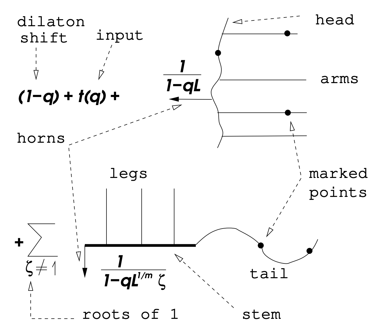
We will now explain Figure 4. Let be the cotangent line at the first marked point and let be the automorphism of a point of . Then is defined by the condition that acts on with eigenvalue . In both pictures, the bullet denotes the first marked point and its image in , while a thick component is one which is a multiple cover of its image.
First, suppose that . Then the black component is the maximal connected component containing the first marked point on which acts as the identity. The red and blue components are precisely those on which acts nontrivially, and we refer to them as arms.
Now suppose that is an -th root of unity for some . In this case, the nodes of the black component are required to be balanced with respect to the -action, so we cut off the nonbalanced part, which is colored blue, and refer to it as the tail. On what remains, the black component is the maximal connected component containing the first marked point on which acts as the identity. Finally, after taking out the black component and the tail, we refer to the remaining components as legs.
The following definition is due to Givental. We write
where the term is simply the contribution of under the Riemann-Roch theorem. Now, we will define arms, legs, and tails. Here, we define the arms
the legs
and the tails
Proposition 5.37 ([GT14]).
The Laurent expansion of the J-function at is given by
where the fake invariants are computed by applying Riemann-Roch and only considering the contribution of the untwisted sector.
Proposition 5.38 ([GT14]).
At any other root of unity , we have
where the stem is some fake invariant of defined on the moduli space
It is defined by the formula
where denotes the normal bundle of .
Remark 5.39.
If we can calculate the fake and stem theories, then we can compute genus zero quantum K invariants.
5.10 Quantum K-theory of a point.
One natural question is to study higher genus quantum K-theory. We will begin with the simplest target, which is a point. One motivation for studying higher-genus would be to try to prove integrality of the Klemm-Pandharipande definition of GV invariants for Calabi-Yau fourfolds or the Pandharipande-Zinger definition of GV invariants for Calabi-Yau fivefolds (in this situation, we only need to consider genus ). One reason we need to consider the quantum K-theory of a point is because in , there are some components where an entire curve of genus is contracted to a point.
Question 5.40.
What is the K-theoretic Witten-Kontsevich theorem?10
We will first recall the cohomological Witten’s conjecture. We will begin with the operator
and deform it to
where we should think of and . Formally, write
using the property
for all integers . In particular, we construct the (2-)KdV hierarchy by the equation
for all . We define a -function to be a function such that
Now perform the above process using . Define the function
Note that because the genus is determined entirely by the number of insertions and the degree of the insertions, the notation
uniquely determines a descendant GW invariant of a point.
Theorem 5.41 (Kontsevich [Kon92]).
is a -function of the KdV hierarchy constructed starting with under the change of variables .
One application of this theorem is to consider virtual localization. For example, suppose we consider where is a unique rational curve in a Calabi-Yau threefold with normal bundle . Then in this setting we can reduce to the local model and compute
via virtual localization. If we would like a similar result in K-theory, then we will need to consider terms of the form
so we will need to consider the permutation-equivariant quantum K-theory of a point.
We now proceed with a literature review. First, Lee [Lee97] computed the formula
Later, Lee–Qu [LQ14] gave a way to compute
in principle. Givental [Giv17] computed the formula
Finally, Milanov [Mil25], in a preprint first posted in 2024, computed
The following pluri-Hodge recursions and the new genus-one calculations based on them are due to You-Cheng Chou and were presented in this lecture.
Let and define the pluri-Hodge sheaf . Considering the map , we will denote the upstairs cotangent lines by and the downstairs ones by .
Lemma 5.42.
For all integers and , we have
Remark 5.43.
Note that if , then . The reason is that this operation sends to .
Proof.
When all are zero, we see that
by Serre duality. The next step is to show that
Here, we first consider the exact sequence
and twist by to obtain
and then compute the pushforward. □
Lemma 5.44.
Let be rational functions, for example . Then
where and .
To prove this, we need to consider the pushforward
Here, we use the fact that and . Applying the previous lemma, we see that the pushforward becomes
Now, Lee’s formula computes the correlators
via the expansion
Note here that there is no Hodge bundle in genus , so in fact the lemma can be used to obtain Lee’s formula.
Lemma 5.45.
We have
The lemmas collectively imply that we can reduce to the case of a single marking at the cost of making the insertions very complicated and introducing pluri-Hodge terms everywhere. In genus , life becomes easier because on , we have
In this case, recall the classical formula
Unfortunately, computing
is too hard, so we can try to compute
which is known, but it is unclear how to write a good formula for it. The reason we would consider this is the operation
Unfortunately, You-Cheng does not know how to write
in a nice form. In principle we can write formulae like
but this does not seem to help much.
5.11 Permutation-equivariant theory of a point.
We can compute in another way. Consider the involution on an elliptic curve, which gives a map
Then, Givental [Giv17] computes
In particular, we obtain
and then because the map is a -gerbe (or a -cover on objects), we obtain the desired formula.
Consider to be the hyperelliptic locus. Note that the marking lies on a Weierstrass point. Note that the fixed points of the hyperelliptic involution go to points on , and therefore one would want to use the calculation
to compute the quantity . However, because of the way that the curves upstairs degenerate, we will need to consider the Hassett moduli space [Has03] where the last markings have weight .
6 Quasimap wall-crossing (Yang Zhou)
The main wall-crossing theorem and master-space construction in this lecture are from [Zho22]. Earlier genus-zero and higher-genus results appear in [CK14; CK20], and the foundations of stable quasimaps are in [CKM14].
Let be the quintic threefold. Our goal is to count genus zero curves on , which is a problem that was solved by Givental and Lian-Liu-Yau. Via the closed immersion , we can write
which is smooth and has a torus action by . If a map is fixed by this action, the domain must have some components which map to the fixed points and some components which form an cover of the -dimensional orbits. In particular, the fixed locus is indexed by a set of graphs.
In this setting, we have the quantum Lefschetz principle, which states that
Here, the vector bundle is defined by
where is the universal curve and is the universal stable map. We will give a different perspective on the result that if
then
up to the mirror map .
6.1 Naive counting.
We will consider “maps” from a fixed . For simplicity, we will assume is the Fermat quintic. This is given by a collection where such that and . To be an actual morphism, we need the to have no common zeroes, but this moduli is not proper, so we relax this condition. Then we consider the moduli space
This lives inside the corresponding moduli space
of rational maps to projective space. There are two problems. First, the domain is parameterized, so we need to account for the automorphisms of . Second, to obtain stable maps, we need to blow up the domain.
First, let act on by scaling . Consider the special fixed locus defined by
Therefore, . From this perspective, we can rewrite the I-function as
using standard arguments in deformation theory. This lives in .
6.2 Wall-crossing without rigor.
Second, consider a nodal curve with a marking plus a tail with an action of and suppose we have a map . If we take the limit
we see that the limit of the bubble lands in , where the common zero is away from the node. Then we can replace this tail by a new marking which carries some terms of the I-function. For the quintic, this is simply . At the end of this process, we are left with with various contributions of the I-function.
Note that if we consider acting on , then is fixed if for all , there exists such that
commutes. Therefore, we obtain an action of on the domain.
We will define the moduli space of -stable quasimaps to , which is analogous to the moduli of stable maps. We want to think of these moduli spaces as being virtually birational to each other, and each of these is a proper DM stack with perfect obstruction theory, and therefore we can define quasimap invariants
Here, is a positive rational number. The space of possible has a wall and chamber structure, where the walls occur at for positive integers . When we obtain Gromov-Witten theory (namely stable maps), and as we move to the left, we allow fewer rational tails but more basepoints. Eventually, in the limit, no rational tails are allowed. In the end, we obtain the following wall-crossing formula around the wall at :
Here, . In the special case, where , , and , we obtain
Crossing all walls from the GW chamber, we obtain
which produces the mirror map via the dilaton and divisor equations.
6.3 Quasimaps.
Definition 6.1.
A prestable quasimap to the quintic threefold consists of
where is a prestable curve, , and , such that
is finite and away from the special points. In addition, we require that .
Importantly, we will refer to as the set of base points. Away from , we have an actual morphism . Geometrically, suppose we have a family over where in the limit as , the zero loci will end up colliding. We can either preserve this quasimap in the central fiber, or we can blow up the central fiber some number of times to obtain an actual morphism at the cost of bubbling out a rational tail. Therefore, any moduli space of prestable quasimaps cannot be separated, so we must consider some kind of stability condition.
Definition 6.2.
A prestable quasimap is -stable if
- (1)
For all , we have , where ;
- (2)
The -line bundle has positive degree on every irreducible component of .
Note that for all irreducible components , we have . Therefore, the things which change are curves of genus with special points or curves of genus with no marked points. Note that in the and cases, we have , and in the case, stability is equivalent to , so in the case, the second condition is equivalent to
Example 6.3.
In the chamber, note that the first condition implies that there are no basepoints, and the second condition implies that all unstable components have positive degree, and therefore we have recovered stable maps.
If we move into the chamber where , then we must contract rational tails of degree . For example if we have a chain of two degree rational curves ending in a tail, then we contract the outermost tail and are left with a single degree rational tail with a basepoint of length .
If we move into the chamber, then we must contract all rational tails of degree and replace them with basepoints of length .
Remark 6.4.
In the case of projective space, there is an actual morphism
For a general target, this is not possible, but this idea gives intuition for the phenomenon of quasimap wall-crossing.
We will now discuss how to generalize this to more general target spaces. Let
where is affine, is reductive, and is a character of . We need to require that
- (1)
;
- (2)
has at worst lci singularities and is smooth.
Note that we require the stable locus to have finite stabilizers. For convenience, we will also require
- (1)
is projective;
- (2)
acts freely on the stable locus.
Example 6.5.
In the case of the quintic, is the affine cone over the quintic. The unstable locus consists of the origin, which is the unique singular point.
Example 6.6.
Another example is that we can consider with generic stability condition and obtain a toric variety.
Example 6.7.
We can consider the Grassmannian
where the unstable locus consists of matrices with rank strictly less than .
Remark 6.8.
The condition on the stable locus is always satisfied when is abelian for generic stability conditions, but for non-abelian this is not always possible.
Remark 6.9.
For a general smooth projective variety, the origin is not necessarily lci, so it is unclear how to define quasimaps in a way where we can still define a virtual cycle.
Definition 6.10.
A prestable quasimap to is a map such that the base locus
is finite and away from the special points. By definition, consists of a principal -bundle together with an equivariant map , which is equivalent to a section of the associated bundle .
Example 6.11.
For the quintic, this exactly recovers a line bundle (which is equivalent to a -torsor) combined with a section of which satisfies the defining equation.
In order to define degrees, we can consider the line bundle on . Then we can define the degree of under to be
Example 6.12.
In the example, note that a principal -bundle is equivalent to rank vector bundle on . Therefore, is equivalent to the data of , and therefore quasimaps to the Grassmannian are equivalent to stable quotients. In this case, we are looking for generically surjective
and because , we see that .
Example 6.13.
Consider and note that . If we consider , then we have
However, if we consider , then we have
Here, we see that the scheme structure is sensitive to the choice of character, so we cannot simply naively define the length of a basepoint. Note that
In particular, we must define
Example 6.14.
Let . Then a prestable quasimap is simply
where is finite and away from the special points. In addition, if , we have precisely recovered the data of a new marked point in .
Example 6.15.
Now consider . Also suppose that the degree is . Now we will set
Therefore, note that
Because these all live in degree , we see that for a smooth point , we have
If we set , then the condition that is equivalent to requiring that
The degree condition now states that
Equivalently, this states that
so we recover a weighted pointed curve with weights .
6.4 Master space.
The proof uses virtual localization [GP99]; Hassett's weighted moduli spaces [Has03] provide one of the models for the construction.
Our method will be to perform virtual localization on a master space which interpolates the two moduli. Consider the -action on given by
The fixed loci consists of a where and a point . Then we can compute
by transfering the computation to the other fixed locus. In particular, we lift to and compute
Taking residues, we see that
which recovers the desired integral. The key fact we used here is that projective space is proper.
Example 6.16 (Second toy example).
We will consider a second toy example. Recall Hassett’s moduli of weighted pointed curves
where is nodal and the can collide. The collisions are regulated by the fact that each marked point is given a weight and are required to satisfy the following conditions:
- (1)
For all , then
- (2)
We have the stability condition . For example, if we have a rational tail, then .
Example 6.17 (Another toy example).
Our goal will be to once again compute
Our first goal will be to change the stability condition. If we set
we see that the stability condition does not change. However, if we set
the moduli space does not change, but the universal curve in fact becomes with the section being the diagonal. This tells us that
and we will use this to compute in the chamber. We can try to form a master space by both allowing rational tails with and allowing , but if we do this, we end up with a semistable point with a rational tail where . We want to end up with this by taking a quotient from a master space, so we will add the data of a tangent vector to the moduli. Therefore, define the master space to consist of objects of the form
where is nodal, are smooth points, are disjoint,
for all rational tails , if , then is disjoint from the other , and when , there are no rational tails where for .
We now give this master space an action of by scaling . There are various fixed loci:
- (1)
When , we obtain ;
- (2)
When , we obtain ;
- (3)
There are fixed loci where and we have a rational tail with .
If we consider a general point (with all four marked points disjoint), it will travel directly to itself along the -action. However, if we start with a rational tail containing and , then we first travel to a rational tail with general but , and if we smooth out the node, we obtain a single curve with , but we allow , which is another fixed point. Now we can integrate
Taking residues at , we obtain
where in the final term the in the denominator are node smoothing parameters, and therefore we recover the desired integral.
With all of our toy examples, we are finally ready to discuss the quasimap master space. Our first step at the wall is to allow both degree rational tails and length base points. However, we can consider curves with a rational tail and a quasimap of the form
which have infinitely many automorphisms. However, we cannot attach tangent vectors to the base points (because deformations will remove them), and there are also situations where there exists more than one degree with a base point of length (and then the automorphism group contains ).
Remark 6.18.
There is a key observation. Suppose that we have two rational tails of degree and call the two nodes and . Now define the space of smoothing parameters
where is the rational tail and is the rest of the curve. We will consider the moduli
of weighted semistable curves labelled by degrees. Note that this morphism is highly non-separated. We will consider the open substack where the curves have no tail of degree strictly less than . Then we can consider the Cartier divisor where there exists at least one tail of degree . In particular, we see that
for the two branches and at the point of interest. We also see that , so we can add the data of
and the data of
The actual construction proceeds as follows. Consider . Define to be an iterated blowup along strata of . Then an object of the master space (a quasimap with calibrated tails) over a scheme is given by the data of a quasimap
inducing a morphism , a choice of a lift
a line bundle , and where and , where is nonvanishing. We also disallow basepoints of length strictly larger than and require stability such that
- (1)
When , we obtain -stability;
- (2)
When , we obtain -stability;
- (3)
Any constant tail (degree with base point of length ) is an entangled tail. Here, we consider the last blowup such that maps to an exceptional locus , and then the are entangled tails for ;
- (4)
If there exists a degree tail, then all length base points are on degree tails.
7 Log GLSM (Qile Chen)
Let be a smooth projective variety (or even a DM stack). Let be a vector bundle on with a section which defines a smooth zero section of the expected codimension. We will refer to and as ambient and and as the complete intersection.
Question 7.1.
What is the relationship between the GW theory of and the GW theory of ?
When , Givental and Lian-Liu-Yau used this relationship to compute the GW invariants of complete intersections, and when , this was done by Zinger. In general, there are two approaches: (N)MSP and log GLSM. In this series of lectures, we will discuss log GLSM.11
7.1 R-maps.
We will consider the R-torus . This has a weight representation, which we will call . It descends to a line bundle on . The targets of R-maps will be stacks
which are DM-type, separated, and (log) smooth. Now, an R-map consists of a (2-)commutative diagram
Here, the curve could be prestable, twisted, log, or even punctured.
Example 7.2.
Our first example is that of stable maps. Let . Because in the diagram
the vertical arrow is the second projection, we see that this reduces to a map to .
Example 7.3.
Consider maps
If we assume that is unmarked, we see that the data of this map is simply a section of , and therefore we recover holomorphic differentials.
Example 7.4.
Consider a morphism given by . Then we see that
Now a diagram
with unmarked is equivalent to the data of a line bundle and an isomorphism . Alternatively, we can consider R-maps of the form
which parameterize curves with an R-spin line bundle together with a section.
Example 7.5.
Let be a smooth projective variety. Then consider R-maps of the form
This is equivalent to a map together with a section .
We will consider targets in the GW case. Consider the data of an ambient . Then we will set . The morphism is very nice, but it is not proper. To fix this, we will consider the log stack
Because we have a smooth divisor in a smooth stack, the map is proper and log smooth. Note that we have the zero section
We will now consider targets in the r-spin case. Consider the log stack
This morphism is proper and log smooth.
7.2 Log and punctured R-maps.
We will consider diagrams
where is a log or a punctured (possibly twisted) curve and is an fs log scheme. The stability condition in the GW case is that is representable and
for all and , where is an ample line bundle on the coarse moduli space of . For punctured R-maps, we further require pre-stability.
Example 7.6.
Consider the case of holomorphic differentials. Then consider such that all zeroes are concentrated in a single Weierstrass point, where has genus . If we consider , then the limit consists of a genus component mapping entirely to and a rational component which remembers the zero.
We will now discuss the tropicalization of log or punctured R-maps. Recall that a graph
consists of a set of vertices, a set of half edges, an involution on the half edges, and a root map from half edges to vertices. Then we will let the set of legs be
The edges are pairs of distinct half-edges which are sent to each other by the involution:
Now a decorated graph is a graph combined with a genus function
an assignment
and an ordering
Example 7.7.
For a log or punctured R-map
we will tropicalize it by taking the associated generalized cone complex of the entire diagram. Because has no log structure, what we see is
Now suppose that is a log point with an fs sharp monoid. In particular, this means that . Because everything is (piecewise) linear, it suffices to consider an interior point and consider .
From each half edge, we treat it as pointing outward from the attached vertex, and in particular, this means that a linear map to corresponds to a slope. We will call these contact orders. In particular, we have if are related by . For all , we also define the degeneracy
In particular, is an integral point.
The next thing we need to introduce are punctured legs. They will be denoted by
We will define prestability at such that , which is a technically necessary assumption. Under the assumption that all punctured legs are prestable, we can define the edge length function
Note that is also an integral point for edges . For punctured legs, this is true up to subdivision.
7.3 Log GLSM invariants.
Definition 7.8.
We will define the decorated tropical type of a log map as
Definition 7.9.
A log or punctured map is of compact type if
- (1)
is bounded for all ;
- (2)
for all half-edges with contact order .
We are now able to define the category of stable punctured R-maps fibered over the category of fs log schemes and marked by .
Theorem 7.10 ([CJR21; CJR22]).
The stack is represented by a proper DM stack with basic/minimal log structure.
Remark 7.11.
If is a singleton, then we will write
Consider the diagram
where we set . Then the perfect obstruction theory is defined by
Here, both tangent bundles refer to the log tangent complex. From the perfect obstruction theory, this defines the canonical virtual cycle
The main drawback of this virtual cycle is that it does not reproduce Gromov-Witten theory. However, we can consider how it differs from GW theory, but for this we need a birational modification. Let be a sharp monoid. It has a partial ordering by if there exists a nonzero such that .
Definition 7.12.
We say that either or has uniform maximal degeneracy if there exists such that for all .
Remark 7.13.
If is compact type and has uniform maximal degeneracy, then is uniformly bounded by .
Definition 7.14.
Define to be the stack of stable punctured or log R-maps marked by with uniform maximal degeneracy.
Remark 7.15.
If is a singleton, then we will write
If one of the contact orders is negative, then we will write
Note that there are two types of vertices: if a vertex is mapped to , then either there is at least one half-edge which points upwards or all contact orders are , in which case all are contracted. These are called log vertices. The other type of vertex is one that does not go to . Either all half-edges point downwards, or there are some half-edges which point upwards. These are called -vertices. Moreover, the vertices which are compact types are the ones without upwards-pointing half-edges.
If we forget the condition of having uniform maximal degeneracy, then there is a map
which is a subcategory over . However, as a morphism of algebraic stacks, it is log étale, proper, and surjective. In addition, has a canonical perfect obstruction theory which is pulled back from . In the case when the set of vertices is a singleton, we have
In the case of a log vertex, we in fact have inclusions from the moduli of stable maps with p-fields as
If we denote the moduli of p-fields by , then the boundary
is a Cartier divisor. By the condition of having uniform maximal degeneracy, we have a section
This is equivalent to the data of a morphism
which pulls back to .
We will define a superpotential to be a function
Its critical locus is denoted by
We say that has proper critical locus if is proper.
For example, suppose we are interested in GW theory. Let be a smooth projective variety, be a vector bundle on , and . Set . Then we obtain
Lemma 7.16.
has proper critical locus if and only if is smooth of expected codimension.
Example 7.17.
Let be a point, , and . Then , so the critical locus is empty.
Using the Kiem–Li method of cosection localization [KL13], we can obtain a virtual cycle
which is supported on the critical locus. In GW theory, this equals the GW virtual cycle,
where the sign can be explicitly calculated.
Theorem 7.18 ([CJR21; CJW21]).
Let be of compact type. In the compact type setting,
- (1)
has a reduced perfect obstruction theory, which yields a reduced virtual cycle ;
- (2)
has a reduced perfect obstruction theory, which yields a reduced virtual cycle ;
- (3)
We have in the case of a single log vertex. Moreover, there is the formula
where is the pole order of along .
7.4 Tropical decomposition and finite generation.
The tropical decomposition and its applications below are from the working draft [CJR25]. The effective invariants and their axioms are developed in [CJR22].
From now on, we will consider a simpler setup where is a smooth projective variety and is a line bundle on . In this case, we will assume that is smooth of codimension . Moreover, we will assume that is a Calabi-Yau threefold. We will consider the invariants
and the generating series
Conjecture 7.19 (Yamaguchi-Yau, Alim-Länge [YY04; AL07]).
Suppose mirror symmetry holds for . Then there exists a finitely-generated -algebra such that for all , .
Our main goal is the following.
Theorem 7.20 ([CJR25]).
Let be a Calabi-Yau threefold hypersurface in a Fano fourfold with no odd cohomology. Let be a basis of and be the dual basis. Then for all , we have
Example 7.21.
Let be a toric variety with its toric log structure. Then is the toric fan treated as a cone complex, and we can consider its boundary .
If we consider , we should obtain the similar formula
The question now is what the represent. In fact, they parameterize rigid tropical curves. In the tropicalization
we see that is rigid if and only if the source tropical curve is a bipartite graph with one set of vertices going to and the other set of vertices going to .
Example 7.22.
Let be a point and . Also consider . Then the possible graphs are given in Figure 5.
Theorem 7.23 (Tropical quantum Lefschetz [CJR25]).
Let and be as before. For any , any , and any , we have
Remark 7.24.
There is also a virtual localization formula, announced in [CJR], which can be applied to either the reduced theory (with only the R-torus action) or the canonical theory (which can be applied to the full automorphisms of the ambient space).
Now consider an -vertex. Set and set . Then the first computation is that
where the tropical dimension is . Note that all contact orders are negative, so the second term is at most zero. In particular, we have proved that
Corollary 7.25 ([CJR22]).
If , then .
We also have a balancing condition, which states that
| (1) |
This can be rewritten as
Proposition 7.26 ([CJR22]).
We see that -vertices do not exist in the following cases:
- (1)
We have and is nef;
- (2)
We have and is ample, unless and all .
Definition 7.27.
A marking is a unit if its contact order is .
Notation 7.28.
We will denote the unit sector by and denote , , and .
Theorem 7.29 ([CJR22, Theorems 1.16–1.17]).
- (1)
There is a map , where is birational;
- (2)
We have the equality of reduced virtual cycles;
- (3)
If is a divisor on , then ;
- (4)
Consider the diagram
Then .
Example 7.30.
Consider the setting where and is a hypersurface. We only need to consider and for all . Then we see that
Proposition 7.31 ([CJR22]).
We in fact have
and the equality
Example 7.32.
Now consider the quintic threefold . Then we see that . The unit axiom reduces us to the case when . We must now determine the number of new invariants we need to consider if all , which is equivalent to finding the number of possible . The balancing condition states that
which implies that and therefore that .12
Conjecture 7.33 (Janda [CJR25, Conjecture 1.6]).
- (1)
We have
- (2)
The canonical theory satisfies .
Corollary 7.34 ([CJR25, Theorem 1.7]).
The above conjecture for implies Yamaguchi-Yau finite generation for .
8 Structure of higher-genus GW invariants of the quintic (Shuai Guo)
8.1 The problem.
We will consider the quintic threefold and ask how many curves of genus and degree it contains. In genus zero, the answers begin
Because is Calabi-Yau, the moduli space has virtual dimension zero, and the string equation gives unless . We therefore define the primary invariants by
and we package these numbers in the generating series
The invariants are rational numbers, while the integers we actually want are the BPS invariants . These are defined from the positive-degree part by the multicover transformation
Note that only the are expected to be integral, and that the numbers above are the .
| 0 | 2875 | 609250 | 317206375 | 242467530000 | 229305888887625 |
|---|---|---|---|---|---|
| 1 | 0 | 0 | 609250 | 3721431625 | 12129909700200 |
| 2 | 0 | 0 | 0 | 534750 | 75478987900 |
| 3 | 0 | 0 | 0 | 8625 | |
| 4 | 0 | 0 | 0 | 0 | 49250 |
| 5 | 0 | 0 | 0 | 0 | 1100 |
| 6 | 0 | 0 | 0 | 0 | 10 |
| 7 | 0 | 0 | 0 | 0 | 0 |
We see that every column of Table 2 eventually vanishes. This is the Castelnuovo bound, which for the quintic states that once and was proved by Liu–Ruan [LR22]. Integrality of the entries is the Gopakumar-Vafa conjecture, which was proved by Ionel–Parker [IP18].
In genus zero, Candelas-de la Ossa-Green-Parkes computed using period integrals on the mirror, which we discussed in Section 3.2. In higher genus, Bershadsky-Cecotti-Ooguri-Vafa gave a recursion which produces from the with up to finitely many unknown constants. Our goal is to explain how log GLSM determines this ambiguity.
8.2 Genus zero and the polynomial structure of the B-model.
Recall from Section 3.2 that for the quintic we consider the -function
whose components are annihilated by the Picard-Fuchs operator
If we write and , so that , then the genus zero mirror theorem states that
For our purposes, it is useful to place the quintic formula in the general mirror-symmetry picture. Let be a family of Calabi-Yau threefolds with Kähler moduli and let be a mirror family with complex moduli . The solutions of the Picard-Fuchs equation are periods on and assemble into
which lies in the span of . Here, , , and , and the mirror map is again .
We will use three special points on the complex moduli line of the quintic: the large complex structure point , the conifold point (where a period vanishes), and the orbifold (or Landau-Ginzburg) point . The mirror map is defined at and the expansion there produces Gromov-Witten invariants, while in higher genus we will impose boundary conditions at the other two points.
We now restate the mirror theorem in terms of three-point functions. Pick local coordinates on , let be the corresponding basis on the A-side, and define
Theorem 8.1 (Mirror theorem [Giv98; LLY97]).
We have . Moreover , so it is a globally defined meromorphic function on with poles only along the discriminant.
In particular, after multiplying by the correct power of and applying the mirror map, a genus-zero generating function becomes a rational function of with poles only along the discriminant. Therefore, it is determined by finitely many coefficients.
Example 8.2.
For the quintic in the hyperplane basis,
Example 8.3.
For , the Yukawa couplings are
where
In higher genus, we expect normalized potentials satisfying
where the right hand side is computed by a sum over graphs.
8.3 The BCOV Feynman rule.
The B-model Feynman rule and holomorphic anomaly equation originate in [BCOV94]. For the quintic, Chang–Guo–Li prove polynomiality in [CGL21] and the Feynman rule in [CGL26].
We will now discuss the BCOV recursion as a Feynman rule. It comes from a finite-dimensional model for the quantization of a symplectic transformation as in Section 3.6. Let be symplectic with and set
Given a total potential , we formally define the transformed potential by the Gaussian integral
Expanding by stationary phase gives a sum over graphs. Here, supplies the propagator on each edge and supplies the vertices.
For a Calabi-Yau threefold the propagators are written , , and according to the number of indices, and the vertices are the normalized A-model correlators
Note that these have nothing to do with the operator solving the quantum differential equation, which will appear later.
Example 8.4.
For the quintic in genus two with no markings, the Feynman rule reads
where . This is a cubic polynomial in the propagators.
We can interpret this as a sum over stable graphs, as in Section 3.4. A vertex contributes the lower-genus correlator ; an internal edge contracts two of the insertions against a propagator; the legs record the remaining insertions. Each graph is weighted by . As usual
and is the sum of the contributions of all stable graphs of genus .
8.4 The holomorphic anomaly equation.
We will now rewrite the recursion as a differential equation. The B-model amplitudes are not holomorphic, and for their failure to be holomorphic is given by
Here, is the Yukawa coupling, is obtained from by raising two indices with the Weil-Petersson metric, and is the covariant derivative on the appropriate power of the Hodge line bundle. The two terms on the right are the two boundary strata of , namely a non-separating and a separating node. The forgets the ordering of the two branches.
If we choose local -primitives
so that, modulo a holomorphic term, the anomaly equation becomes the polynomial PDE
These propagators are only defined up to holomorphic tensors, and this freedom is the source of the holomorphic ambiguity.
Remark 8.5.
In the one-parameter normalized variables we will use for the quintic, this reads
To see why the graph sum satisfies this equation, note that in an unmarked potential the non-holomorphic generators occur only in the edge factors. A derivative in a propagator direction therefore picks out a single edge and cuts it. The two half-edges become markings on the resulting lower-genus vertices, and the covariant derivatives correspond to those markings by the divisor equation. We obtain by cutting a loop and by cutting a separating edge.
Remark 8.6.
For clarity, the implication only goes one way. The BCOV graph rule implies the anomaly equation, but the anomaly equation by itself does not determine the graph rule. To recover the same solution, we also need the propagator convention, the lower-genus vertex data, and the boundary conditions.
If all lower-genus vertices are known, then the right hand side is known, so we can integrate with respect to the non-holomorphic generators to obtain
where finite generation gives the holomorphic ambiguity
We see that the anomaly equation leaves unknown coefficients in each genus.
Remark 8.7.
For the quintic, the degree-zero data together with orbifold regularity remove of these freedoms and the conifold gap supplies further conditions, so that
parameters remain and are genuinely new effective invariants. This is exactly the number of -vertex unknowns predicted by Equation 1, namely the number of with .
We therefore obtain the following conjectural algorithm proposed by physicists: the BCOV Feynman rule, orbifold regularity at the Landau-Ginzburg point (a form of the LG/CY correspondence, which for the quintic is work in progress of Guo-Ruan-Janda), and the conifold gap condition. To these we may add the Gopakumar-Vafa integrality and the Castelnuovo bound.
8.5 Four theories.
Recall from Section 7 that the log GLSM carries two virtual cycles. The reduced cycle recovers quintic Gromov-Witten theory, while the canonical equivariant cycle admits a root of unity specialization which is semisimple and therefore computable by Givental-Teleman. The bipartite graph sum
expresses the former in terms of the latter, at the cost of introducing the effective invariants at the -vertices. Replacing these by formal parameters gives the extended -family, whose vertex data is supplied by the meromorphic and rubber log GLSM theories.
We will consider the following four theories.
- •
The -twisted geometric theory sets and keeps the auxiliary weight . It has both stable-map and stable-quotient versions, and the quotient version gives the genus two localization formula below.
- •
The formal quintic, or formal -twisted theory, sets and . It is a semisimple CohFT, so it has a universal and computable -matrix.
- •
The extended -family interpolates between these, and is where bipartite graphs with both formal and meromorphic vertices live.
- •
Quintic Gromov-Witten theory is obtained by setting and then letting , and is the theory we want to compute.
Warning 8.8.
In higher genus the coefficient of the -twisted stable quotient theory is not the coefficient of the formal -twisted theory.
8.6 The formal quintic.
The formal quintic and its holomorphic anomaly equations are studied in [LP19]; the comparison with the extended theory is developed in [GJR18].
Let and let be the universal curve. The -twisted cycle is
where has equivariant first Chern class . Starting instead from the fully -equivariant cycle, the formal quintic is the root of unity specialization
where . The relation makes the quantum product generically semisimple while retaining as a parameter.
The state space, unit, and pairing are given by
and the CohFT classes are
where forgets the map and stabilizes the domain. If we shift by with , then the shifted theory is semisimple. After extending scalars to , the idempotent basis satisfies
Then Theorem 3.24 gives
with the decorations of Section 3.4. A leg carrying gets , an edge gets
and a vertex gets the topological field theory , with the missing unit-preserving part inserted at forgotten markings via .
Remark 8.9.
We see that the edge factor has no pole. Setting and using the symplectic condition in the form , the numerator vanishes. Therefore, it is divisible by , and is a power series in the two cotangent line variables. The coefficient of is the class placed at a node with , and contracting it against the two adjacent topological field theory tensors glues the branches.
8.7 How to compute the -matrix.
To compute the -matrix, we begin with the formal equivariant -function
The coefficients through are independent of , so and the mirror shift is free of logarithms. Set
and introduce the bases
where the diagonal Birkhoff factors are defined recursively by
so that in particular . The idempotents and canonical coordinates are given by
We will use the quantum differential equation to determine the -dependence of the -matrix. The fundamental solution satisfies
and in the normalized canonical direction the stationary phase asymptotics give
so that
Here, is the quantum Riemann-Roch (equivalently, Gamma function) factor, and together with the symplectic condition it fixes the constants that the differential equation cannot see. As at the end of Section 3.7, the differential equation gives a recursion and an oscillating integral gives the initial conditions.
Writing , we can use the equation above to determine each from the preceding ones. There are two features which make the quintic tractable. First, the root of unity basis has five sectors, and a mod charge rule permits only one residue pattern in each row. Then most matrix entries vanish before any computation starts. Second, every coefficient lies in the finitely generated ring
so the stable graph sum reduces to a finite algebraic computation.
Remark 8.10.
In particular, a fixed genus only needs finitely much of for dimensional reasons. On only classes of total degree at most contribute and everything else integrates to zero, so for an unmarked potential we need only . Genus stops at and genus at .
8.8 Genus two.
The genus-two mirror formula discussed here is due to Guo–Janda–Ruan [GJR17].
We will now carry out both routes in genus two. The geometric route uses the -twisted stable quotient theory, applies virtual localization to get five contributions, and then applies stable quotient wall crossing to land on quintic Gromov-Witten theory. The formal route uses the semisimple -twisted theory and the -matrix to compute a stable graph sum. This gives only the formal leading part. Then the effective and meromorphic rest graphs must still be added.
Notation 8.11.
Write
where is the universal stable quotient line bundle and (a sign convention we return to below). This is the stable quotient sign convention, and is not the same as the appearing in the stable map cycle above.
The four non-constant graphs are drawn in Figure 6, and their contributions are
and, writing and for the double edge graph,
Note that these correlators live on , so is present and nonzero.
There is a fifth contribution from the degree zero graph, which is the constant
and adding the five contributions, we obtain the localization identity
where the two factors of are the automorphisms of and .
Set and , where is the ordinary mirror shift. We now apply stable quotient wall crossing to obtain the exact identity
Introducing and the generators
the individual twisted graph contributions involve extra generators. The important point for us is that these cancel in the above linear combination and leave precisely the finite generation variables. Writing and , we obtain
If we expand at large radius, then we obtain
and these coefficients are the Gromov-Witten invariants , not the BPS integers of Table 2.
We now turn to the formal route. The Givental-Teleman formula for is a sum over the seven stable graphs of genus two with no legs, which are drawn in Figure 7. Only through is needed, and the translations expand the seven topologies into decorated strata.
Remark 8.12.
These are dual graphs of stable curves and are not the graphs of Figure 5, which are the rigid tropical types obtained by applying the tropical decomposition formula to the reduced theory of the log GLSM. The two lists of topologies happen to coincide here, but a vertex means something different in each. Here it is a component of the domain curve carrying a topological field theory tensor. There it is a level of a bipartite tropical curve carrying either a log or an -vertex moduli problem.
For the formal route, we define the normalized potential intrinsically by
The complete graph sum lies in and equals
For clarity, this is the exact formal -twisted answer and is not . Note also that is the discriminant generator while is a logarithmic derivative generator.
8.9 Finite generation and the extended family.
Recall the finitely generated ring from above, which we will grade by
For as before, set
Theorem 8.13 (Graded finite generation [GJR18]).
We have
Consequently, after assembling the bipartite rest graphs, the non-equivariant component of the extended family satisfies
In particular, at each fixed only finitely many graded monomials can appear, and only -matrix orders up to can contribute.
We organize the extended theory using the bipartite graph sum
where is an effective or meromorphic vertex factor, is a formal zero-vertex correlator, the and record incident degrees, and is the edge factor. The limit is taken only after the complete graph sum. Setting leaves the formal -twisted leading sector. Setting and recovers quintic Gromov-Witten theory. Differentiating a universal edge cuts it and produces the holomorphic anomaly equation, while leaving the effective vertices untouched.
To derive the holomorphic anomaly equation, write and introduce
together with the two non-holomorphic directions
Theorem 8.14 (Holomorphic anomaly equation for the extended family [GJR18]).
We have
We prove this by the cutting argument of Section 8.4, which works because the derivative of the -matrix propagator is simply
Derivatives of and of every edge remain inside the same graded ring, so cutting a differentiated edge closes up on lower-genus correlators in . If we set , then we recover the same equations for the formal -twisted theory.
8.10 Boundary conditions.
We will use two sources of conditions on the holomorphic ambiguity.
First, we use regularity at the orbifold or Landau-Ginzburg point , equivalently . For either the formal or an assembled extended potential , set
Theorem 8.13 bounds the possible Laurent powers of , and the formal LG/CY identification says that after analytic continuation and identification of the normalized CY and LG bases, the same formal -matrix polynomial describes both phases. Therefore
and for with the quintic bound is
Note that this is a statement about the assembled normalized graph contribution, and not about individual bare meromorphic or rubber vertex correlators.
Second, we study the conifold. Set
where form a local conifold period pair normalized so that the vanishing flat coordinate satisfies at the conifold. Given a rational expression in the finite generation data, we obtain its conifold value by substituting the Laurent expansions of all generators as series in . Theorem 8.13 gives the pole bound
but what we need is the stronger gap condition
namely that every intermediate negative power vanishes. This is conditions and is not implied by finite generation.
Conjecture 8.15 (Formal conifold gap).
The formal -twisted potential has the universal leading term
where is a Bernoulli number.
Example 8.16.
In genus two the computed expansion begins
This is the genus two gap, not merely the pole order bound.
We must also consider the formal correlators with rational descendant insertions which occur in the rest graphs, namely
with and .
Conjecture 8.17 (Regularity with special insertions).
We have .
For fixed and , individual terms in the -expansion may have poles. Note that the assertion concerns the complete rational descendant insertion, whose negative powers cancel before the rest graph sum over is taken. It is a statement about these specific formal correlators rather than about every unassembled meromorphic correlator.
We can use Conjectures 8.15 and 8.17 to transfer the gap to quintic Gromov-Witten theory. A rest graph contribution has the shape
and the factors are finite polynomials in , so they are conifold regular. Then the formal leading gap together with regularity of the special correlators implies the gap for the extended family, and therefore for the quintic.
Remark 8.18.
Conjectures 8.15 and 8.17 are open in general, but have been verified for the quintic through by Guo-Janda-Ruan. The pole bound for the extended family is a theorem, and the gap follows from the two conjectures and is proved for by explicit computation. At the time of these lectures, the all-genus gap for quintic Gromov-Witten theory was therefore conditional on them and unconditional for .13
Putting all of this together, we begin with the Picard-Fuchs data and compute the Givental -matrix and the operator . We then obtain the formal stable graphs and meromorphic rest graphs, use the holomorphic anomaly equation and finite generation, and finally impose the orbifold and conifold boundary conditions to determine .
9 Structure of higher-genus GW theory of local (Shuai Guo)
This lecture is based on joint work with Jingyi Xu and Qingsheng Zhang.
9.1 The geometry of .
We will consider the total space
which is a non-compact toric Calabi-Yau threefold. For this is the resolved conifold.
Let be a lattice of rank and let be the dual lattice, which we identify with the characters of . The one-dimensional cones of the fan of are generated by
and contains as an open dense subset. Using the dual vector we obtain the Calabi-Yau subtorus
whose action preserves the Calabi-Yau form. The toric graph consists of two triangles, which correspond to the two fixed points of the torus action. The weights of the -action at the first fixed point are
and at the second fixed point they are
We can therefore express the invariants in terms of equivariant cohomology by localizing at these two fixed points. Here, .
Unfortunately, for the toric graph of is not convex. Then is not semiprojective. This is the reason the case at hand is not covered by the existing literature, as we will explain in Section 9.5.
9.2 The conjecture of CGMPS.
In 2007, Caporaso, Griguolo, Mariño, Pasquetti, and Seminara studied the Gromov-Witten theory of . Writing
for the total free energy, they computed the genus-one part exactly and proposed the ansatz
| (2) |
for . Here, the variable is related to the Kähler parameter by and . Our convention will differ by for .
Analyzing the asymptotics of the genus-zero invariants, CGMPS defined the scaled string coupling by
and introduced the double-scaling limit , which is obtained from by letting and with fixed. Combining their genus-zero and genus-one results with the ansatz gives
where .
Conjecture 9.1 (CGMPS [Cap+07]).
The double-scaling limit coincides with the free energy of the minimal model.
The free energy of the minimal model has the form
where
so we see that Conjecture 9.1 is equivalent to the statement that for all .
9.3 The main results.
The global mirror symmetry picture of Section 8 applies here as well. Our goal is to describe the behavior of at the three boundary points of the one-dimensional B-model moduli space. The limit is the large complex structure limit and gives the Gromov-Witten expansion in the A-model variable . At , we will use the framed -matrix to prove that remains regular. The interesting point is , which is a higher-order critical point. Unlike an ordinary conifold singularity, whose genus- leading pole has order , this degeneration has pole order at most . Its leading coefficient is governed by the minimal model.
Theorem 9.2.
For any integer and any , the Gromov-Witten potential of is computed by the Eynard-Orantin topological recursion of a spectral curve , namely
In particular, this gives a non-semiprojective toric Calabi-Yau example of the remodeling conjecture.
Theorem 9.3.
For , the potential is the expansion of a rational function
where .
In particular, this proves the structural ansatz Equation 2.
To identify the double-scaling limit, it remains to determine the constant term of at .
Theorem 9.4.
The constant term of is
9.4 Gromov-Witten theory of .
For the equivariant theory of local curves and its localization formulas, see [BP08].
Because is noncompact, the moduli space is not proper and the degree of the virtual class is not defined a priori. To define the invariants, we will introduce a torus action and pass to a twisted theory on , where we can apply virtual localization.
We choose a framing and let . The two localized weight rows, each of which includes one zero weight, are
If , then rescaling the character gives an equivalent symmetric weight vector
and we denote the adjusted torus by . If , this normalization is
Let be the forgetful map and let be the evaluation at the marking. Then we define
where is the equivariant Euler class. For this specializes to the usual resolved conifold formula.
We obtain a CohFT with state space the equivariant cohomology ring
and pairing
In the flat basis the Gram matrix is given by
We define the correlators by
where is the forgetful map to . The twisted virtual class is given by
Set . Then the genus- potential is given by
Remark 9.5.
The degree-positive invariants are independent of by the topological vertex [LLLZ09], and their -independence also follows from Theorem 9.8. We will use the -independence in the proof of Theorem 9.3.
In genus zero, we have
which allows us to compute the Yukawa coupling exactly:
Here, and are related by the mirror map . Evaluating the quantum product using , we obtain
or in matrix form
The eigenvalues of this matrix are generically distinct. Then is semisimple. We write for the idempotent basis, for the lengths, and for the normalized canonical basis.
Because the theory is semisimple, Theorem 3.24 gives
where is a one-dimensional trivial CohFT and with . We determine the -matrix from the quantum differential equation
Equivariant localization and quantum Riemann-Roch relate the fundamental solution to the -matrix by
where the initial condition is an exponential involving Bernoulli numbers. Writing , we obtain from the quantum differential equation the second-order equation
where . We can then compute the -matrix order by order in .
9.5 Topological recursion and the remodeling conjecture.
We now pass to the B-model side. Our goal is to identify the reconstruction supplied by topological recursion with the Givental-Teleman reconstruction above. The Eynard–Orantin topological recursion [EO07] takes as input a spectral curve , where is a Riemann surface; is locally defined with meromorphic differential having finitely many simple zeros; is holomorphic near those zeros, with there; and is a fundamental bidifferential on . Near a zero of , let be the local conjugate point with and define the recursion kernel
If we set , , and , then the multi-differentials are defined recursively for by
where the primed sum excludes . For the free energy is given by
The remodeling conjecture [BKMP09] of Bouchard, Klemm, Mariño, and Pasquetti asserts that the all-genus open and closed Gromov-Witten invariants of a toric Calabi-Yau threefold coincide with the invariants produced by topological recursion on its mirror curve. It was proved for , the resolved conifold, and local curves by Eynard-Orantin, Zhou, and Chen-Li-Liu. Then Fang–Liu–Zong [FLZ20] proved it for all semiprojective toric Calabi-Yau threefolds. Unfortunately, is not semiprojective for , so it falls outside the scope of that proof.
To compare the two sides we use the reconstruction of Dunin-Barkowski, Orantin, Shadrin, and Spitz [DOSS14], which identifies the stable topological recursion correlators with the Givental reconstruction of a semisimple CohFT. Around each critical point , define the local Airy coordinate by
and the globally defined meromorphic reference form
The state space of the associated CohFT is spanned by the basis corresponding to the critical points, and the pairing is diagonal with . The curve -matrix is defined by the asymptotic Laplace transform
and the analogous transform of defines , and if the resulting CohFT has a flat unit, then . Then is symplectic, the curve CohFT is , and writing , the correspondence reads
For , we will consider the spectral curve
where
Solving , we obtain the critical points
and the inner products are given by . Then the resulting lengths satisfy . Therefore, the Frobenius structure of the spectral curve is the quantum product of .
We have now matched the Frobenius structures, so it remains to match the two -matrices. Integration by parts on the Lefschetz thimbles gives
where
are exactly the entries of the quantum product computed above, so these agree with the quantum differential equation for the Gromov-Witten -matrix. To match the initial conditions, we take the limit of the Laplace transforms along the thimbles, which produces Beta functions and therefore products of Gamma functions. Then Stirling’s expansion matches the Bernoulli-number initial condition .
Proposition 9.6.
The two -matrices coincide, namely .
We have now shown that the canonical lengths and the -matrices agree. After the substitution , the genus- stable graph sums differ by the overall parity , which proves Theorem 9.2.
9.6 Rationality.
Because the higher-genus potential is independent of , we may, for simplicity, set . This simplifies both the canonical basis and the quantum differential equation, and the latter becomes
and we denote the entries of the -matrix by . Set
We now use induction on the coefficients of the quantum differential equation to obtain a polynomial structure.
Proposition 9.7.
For and , we have
Analyzing the degree contributions of the stable graph sum in the Givental-Teleman reconstruction, and tracking the powers of , , and , we obtain the following.
Theorem 9.8.
Writing for the codimension- component, we have
Taking and in Theorem 9.8 gives
so Theorem 9.3 will follow if the degree of the numerator in is bounded by . We can see this bound at . Because has a simple pole there, regularity of forces the numerator to cancel the highest powers of . We have therefore reduced rationality to regularity at . This regularity follows from the -independence of together with the existence of the limit of the -matrix for .
9.7 The limit .
To determine the remaining constant term, we now study the limit , which is precisely the double-scaling limit. We rescale the canonical lengths by
and define the modified -matrix entries by isolating the leading terms at in Proposition 9.7, namely
Then the graph sum for becomes a formula for after replacing by and by .
Lemma 9.9.
Solving the leading-order quantum differential equation at gives the closed forms
After factoring out the -dependent terms in Lemma 9.9, we obtain purely rational coefficients. We now construct the topological field theory on with unit , where
Applying reconstruction by together with its flat-unit translation, we obtain a constant with
and it remains to identify the reconstructed CohFT.
The minimal model has spectral curve
with flat coordinate . If we set and and identify and , then the -matrix obtained from at coincides with the -matrix of this curve. Therefore, is exactly the free energy of the minimal model.
Finally, we apply the symplectic swap , under which the curve becomes
The swapped curve has one-dimensional state space, trivial -matrix, and translation , so that
which is Theorem 9.4. Note that this swap is the correspondence between the and the minimal models, which is why the intersection numbers appearing here are those of Conjecture 9.1.
References
- [ACGS25]. Punctured logarithmic maps. Vol. 15. Memoirs of the European Mathematical Society. EMS Press, Berlin, 2025. viii+156. doi: 10.4171/mems/15.
- [ACP15]. “The tropicalization of the moduli space of curves”. In: Ann. Sci. Éc. Norm. Supér. (4) 48.4 (2015), pp. 765–809. doi: 10.24033/asens.2258.
- [AHR20]. “A Luna étale slice theorem for algebraic stacks”. In: Ann. of Math. (2) 191.3 (2020), pp. 675–738. doi: 10.4007/annals.2020.191.3.1.
- [AL07]. “Polynomial structure of the (open) topological string partition function”. In: J. High Energy Phys. 10, 045 (2007). doi: 10.1088/1126-6708/2007/10/045.
- [Alp13]. “Good moduli spaces for Artin stacks”. In: Ann. Inst. Fourier (Grenoble) 63.6 (2013), pp. 2349–2402. doi: 10.5802/aif.2833.
- [BBD82]. “Faisceaux pervers”. In: Analysis and topology on singular spaces, I (Luminy, 1981). Vol. 100. Astérisque. Soc. Math. France, Paris, 1982, pp. 5–171. url: https://www.numdam.org/item/AST_1982__100__1_0/.
- [BCOV94]. “Kodaira-Spencer theory of gravity and exact results for quantum string amplitudes”. In: Comm. Math. Phys. 165.2 (1994), pp. 311–427. doi: 10.1007/BF02099774.
- [BF97]. “The intrinsic normal cone”. In: Invent. Math. 128.1 (1997), pp. 45–88. doi: 10.1007/s002220050136.
- [BKMP09]. “Remodeling the B-model”. In: Comm. Math. Phys. 287.1 (2009), pp. 117–178. doi: 10.1007/s00220-008-0620-4.
- [BM83]. “Partial resolutions of nilpotent varieties”. In: Analysis and topology on singular spaces, II, III (Luminy, 1981). Astérisque 101–102. Soc. Math. France, Paris, 1983, pp. 23–74. url: https://numdam.org/item/AST_1983__101-102__23_0/.
- [BP08]. “The local Gromov-Witten theory of curves”. In: J. Amer. Math. Soc. 21.1 (2008). With an appendix by Bryan, C. Faber, A. Okounkov and Pandharipande, pp. 101–136. doi: 10.1090/S0894-0347-06-00545-5.
- [Cap+07]. “Phase transitions, double-scaling limit, and topological strings”. In: Phys. Rev. D 75.4, 046004 (2007). doi: 10.1103/PhysRevD.75.046004.
- [CG07]. “Quantum Riemann-Roch, Lefschetz and Serre”. In: Ann. of Math. (2) 165.1 (2007), pp. 15–53. doi: 10.4007/annals.2007.165.15.
- [CGL21]. “Polynomial structure of Gromov-Witten potential of quintic -folds”. In: Ann. of Math. (2) 194.3 (2021), pp. 585–645. doi: 10.4007/annals.2021.194.3.1.
- [CGL26]. “BCOV Feynman rule of the quintic threefold”. In: Duke Math. J. 175.4 (2026), pp. 607–675. doi: 10.1215/00127094-2025-0038.
- [CGYZ26]. Conifold Gap for the Quintic Threefold. Preprint. 2026. arXiv: 2609.13921 [math.AG].
- [CJR]. “Structural formulae in logarithmic Gauged Linear Sigma Models III: The localization formula”. In preparation. url: https://fjanda.web.illinois.edu/research.html (visited on 09/16/2026).
- [CJR21]. “The logarithmic gauged linear sigma model”. In: Invent. Math. 225.3 (2021), pp. 1077–1154. doi: 10.1007/s00222-021-01044-2.
- [CJR22]. Punctured logarithmic R-maps. Preprint. 2022. arXiv: 2208.04519 [math.AG].
- [CJR25]. “Structural formulae in logarithmic Gauged Linear Sigma Models I: The tropical decomposition formula”. Working draft. Jan. 6, 2025. url: https://fjanda.web.illinois.edu/Tropical.pdf.
- [CJW21]. “Virtual cycles of stable (quasi-)maps with fields”. In: Adv. Math. 385, 107781 (2021). doi: 10.1016/j.aim.2021.107781.
- [CK14]. “Wall-crossing in genus zero quasimap theory and mirror maps”. In: Algebr. Geom. 1.4 (2014), pp. 400–448. doi: 10.14231/AG-2014-019.
- [CK20]. “Quasimap wall-crossings and mirror symmetry”. In: Publ. Math. Inst. Hautes Études Sci. 131 (2020), pp. 201–260. doi: 10.1007/s10240-020-00114-0.
- [CKM14]. “Stable quasimaps to GIT quotients”. In: J. Geom. Phys. 75 (2014), pp. 17–47. doi: 10.1016/j.geomphys.2013.08.019.
- [CL22]. Quantum K-invariants and Gopakumar–Vafa invariants I. The quintic threefold. Preprint. 2022. arXiv: 2211.00788 [math.AG].
- [CL25]. “Quantum -invariants and Gopakumar-Vafa invariants, II: Calabi-Yau threefolds at genus zero”. In: Geom. Topol. 29.9 (2025), pp. 4665–4693. doi: 10.2140/gt.2025.29.4665.
- [CM02]. “The hard Lefschetz theorem and the topology of semismall maps”. In: Ann. Sci. École Norm. Sup. (4) 35.5 (2002), pp. 759–772. doi: 10.1016/S0012-9593(02)01108-4.
- [COGP91]. “A pair of Calabi-Yau manifolds as an exactly soluble superconformal theory”. In: Nuclear Phys. B 359.1 (1991), pp. 21–74. doi: 10.1016/0550-3213(91)90292-6.
- [Del68]. “Théorème de Lefschetz et critères de dégénérescence de suites spectrales”. In: Inst. Hautes Études Sci. Publ. Math. 35 (1968), pp. 107–126. doi: 10.1007/BF02698925.
- [DOSS14]. “Identification of the Givental formula with the spectral curve topological recursion procedure”. In: Comm. Math. Phys. 328.2 (2014), pp. 669–700. doi: 10.1007/s00220-014-1887-2.
- [EHKV01]. “Brauer groups and quotient stacks”. In: Amer. J. Math. 123.4 (2001), pp. 761–777. doi: 10.1353/ajm.2001.0024.
- [EO07]. “Invariants of algebraic curves and topological expansion”. In: Commun. Number Theory Phys. 1.2 (2007), pp. 347–452. doi: 10.4310/CNTP.2007.v1.n2.a4.
- [FLZ20]. “On the remodeling conjecture for toric Calabi-Yau 3-orbifolds”. In: J. Amer. Math. Soc. 33.1 (2020), pp. 135–222. doi: 10.1090/jams/934.
- [Giv00]. “On the WDVV equation in quantum -theory”. In: Michigan Math. J. 48 (2000). Dedicated to William Fulton on the occasion of his 60th birthday, pp. 295–304. doi: 10.1307/mmj/1030132720.
- [Giv01a]. “Gromov-Witten invariants and quantization of quadratic Hamiltonians”. In: Mosc. Math. J. 1.4 (2001), pp. 551–568, 645. doi: 10.17323/1609-4514-2001-1-4-551-568.
- [Giv01b]. “Semisimple Frobenius structures at higher genus”. In: Internat. Math. Res. Notices 23 (2001), pp. 1265–1286. doi: 10.1155/S1073792801000605.
- [Giv04]. “Symplectic geometry of Frobenius structures”. In: Frobenius manifolds. Quantum Cohomology and Singularities. Ed. by Claus Hertling and Matilde Marcolli. Aspects Math. E36. Friedr. Vieweg, Wiesbaden, 2004, pp. 91–112. doi: 10.1007/978-3-322-80236-1_4.
- [Giv15a]. Permutation-equivariant quantum K-theory II. Fixed point localization. Preprint. 2015. arXiv: 1508.04374 [math.AG].
- [Giv15b]. Permutation-equivariant quantum K-theory VII. General theory. Preprint. 2015. arXiv: 1510.03076 [math.AG].
- [Giv17]. “Permutation-equivariant quantum K-theory I. Definitions. Elementary K-theory of ”. In: Mosc. Math. J. 17.4 (2017), pp. 691–698. doi: 10.17323/1609-4514-2017-17-4-691-698.
- [Giv96]. “Equivariant Gromov-Witten invariants”. In: Internat. Math. Res. Notices 13 (1996), pp. 613–663. doi: 10.1155/S1073792896000414.
- [Giv98]. “A mirror theorem for toric complete intersections”. In: Topological field theory, primitive forms and related topics (Kyoto, 1996). Ed. by Masaki Kashiwara, Atsushi Matsuo, Kyoji Saito, and Ikuo Satake. Vol. 160. Progr. Math. Birkhäuser Boston, Boston, MA, 1998, pp. 141–175. doi: 10.1007/978-1-4612-0705-4_5.
- [GJR17]. A mirror theorem for genus two Gromov-Witten invariants of quintic threefolds. Preprint. 2017. arXiv: 1709.07392 [math.AG].
- [GJR18]. Structure of Higher Genus Gromov-Witten Invariants of Quintic 3-folds. Preprint. 2018. arXiv: 1812.11908 [math.AG].
- [GP99]. “Localization of virtual classes”. In: Invent. Math. 135.2 (1999), pp. 487–518. doi: 10.1007/s002220050293.
- [GS22]. “On the quantum K-theory of the quintic”. In: SIGMA Symmetry Integrability Geom. Methods Appl. 18, 021 (2022). doi: 10.3842/SIGMA.2022.021.
- [GT14]. “The Hirzebruch-Riemann-Roch theorem in true genus-0 quantum K-theory”. In: Symplectic, Poisson, and noncommutative geometry. Ed. by Tohru Eguchi, Yakov Eliashberg, and Yoshiaki Maeda. Vol. 62. Math. Sci. Res. Inst. Publ. Cambridge Univ. Press, New York, 2014, pp. 43–91. doi: 10.1017/9781107297258.003.
- [Hal14]. On the structure of instability in moduli theory. Preprint. 2014. arXiv: 1411.0627 [math.AG].
- [Hal15]. Remarks on Theta-stratifications and derived categories. Preprint. 2015. arXiv: 1502.03083 [math.AG].
- [Has03]. “Moduli spaces of weighted pointed stable curves”. In: Adv. Math. 173.2 (2003), pp. 316–352. doi: 10.1016/S0001-8708(02)00058-0.
- [HN74]. “On the cohomology groups of moduli spaces of vector bundles on curves”. In: Math. Ann. 212 (1974–1975), pp. 215–248. doi: 10.1007/BF01357141.
- [IP18]. “The Gopakumar-Vafa formula for symplectic manifolds”. In: Ann. of Math. (2) 187.1 (2018), pp. 1–64. doi: 10.4007/annals.2018.187.1.1.
- [Kal06]. “Symplectic singularities from the Poisson point of view”. In: J. Reine Angew. Math. 600 (2006), pp. 135–156. doi: 10.1515/CRELLE.2006.089.
- [Kat00]. “Log smooth deformation and moduli of log smooth curves”. In: Internat. J. Math. 11.2 (2000), pp. 215–232. doi: 10.1142/S0129167X0000012X.
- [Kat89]. “Logarithmic structures of Fontaine-Illusie”. In: Algebraic analysis, geometry, and number theory (Baltimore, MD, 1988). Ed. by Jun-ichi Igusa. Johns Hopkins Univ. Press, Baltimore, MD, 1989, pp. 191–224. url: https://math.uchicago.edu/~drinfeld/p-adic_periods/Kato_log-structures.pdf.
- [KL13]. “Localizing virtual cycles by cosections”. In: J. Amer. Math. Soc. 26.4 (2013), pp. 1025–1050. doi: 10.1090/S0894-0347-2013-00768-7.
- [KM94]. “Gromov-Witten classes, quantum cohomology, and enumerative geometry”. In: Comm. Math. Phys. 164.3 (1994), pp. 525–562. doi: 10.1007/BF02101490.
- [KM97]. “Quotients by groupoids”. In: Ann. of Math. (2) 145.1 (1997), pp. 193–213. doi: 10.2307/2951828.
- [Kon92]. “Intersection theory on the moduli space of curves and the matrix Airy function”. In: Comm. Math. Phys. 147.1 (1992), pp. 1–23. doi: 10.1007/BF02099526.
- [Lee04]. “Quantum -theory. I. Foundations”. In: Duke Math. J. 121.3 (2004), pp. 389–424. doi: 10.1215/S0012-7094-04-12131-1.
- [Lee97]. “A formula for Euler characteristics of tautological line bundles on the Deligne-Mumford moduli spaces”. In: Internat. Math. Res. Notices 8 (1997), pp. 393–400. doi: 10.1155/S1073792897000263.
- [LLLZ09]. “A mathematical theory of the topological vertex”. In: Geom. Topol. 13.1 (2009), pp. 527–621. doi: 10.2140/gt.2009.13.527.
- [LLY97]. “Mirror principle. I”. In: Asian J. Math. 1.4 (1997), pp. 729–763. doi: 10.4310/AJM.1997.v1.n4.a5.
- [LP19]. “Holomorphic anomaly equations for the formal quintic”. In: Peking Math. J. 2.1 (2019), pp. 1–40. doi: 10.1007/s42543-018-0008-0.
- [LQ14]. “Euler characteristics of universal cotangent line bundles on ”. In: Proc. Amer. Math. Soc. 142.2 (2014), pp. 429–440. doi: 10.1090/S0002-9939-2013-11800-9.
- [LR22]. Castelnuovo bound and higher genus Gromov-Witten invariants of quintic 3-folds. Preprint. 2022. arXiv: 2210.13411 [math.AG].
- [MFK94]. Geometric invariant theory. 3rd ed. Vol. 34. Ergebnisse der Mathematik und ihrer Grenzgebiete (2) [Results in Mathematics and Related Areas (2)]. Springer-Verlag, Berlin, 1994. xiv+292. doi: 10.1007/978-3-642-57916-5.
- [Mil25]. “K-theoretic Heisenberg algebras and permutation-equivariant Gromov-Witten theory”. In: Int. Math. Res. Not. IMRN 11, rnaf139 (2025). doi: 10.1093/imrn/rnaf139.
- [Ols03]. “Logarithmic geometry and algebraic stacks”. In: Ann. Sci. École Norm. Sup. (4) 36.5 (2003), pp. 747–791. doi: 10.1016/j.ansens.2002.11.001.
- [PPZ15]. “Relations on via -spin structures”. In: J. Amer. Math. Soc. 28.1 (2015), pp. 279–309. doi: 10.1090/S0894-0347-2014-00808-0.
- [Tel12]. “The structure of 2D semi-simple field theories”. In: Invent. Math. 188.3 (2012), pp. 525–588. doi: 10.1007/s00222-011-0352-5.
- [Toë99]. “Théorèmes de Riemann-Roch pour les champs de Deligne-Mumford”. In: -Theory 18.1 (1999), pp. 33–76. doi: 10.1023/A:1007791200714.
- [YY04]. “Topological string partition functions as polynomials”. In: J. High Energy Phys. 7, 047 (2004). doi: 10.1088/1126-6708/2004/07/047.
- [Zho22]. “Quasimap wall-crossing for GIT quotients”. In: Invent. Math. 227.2 (2022), pp. 581–660. doi: 10.1007/s00222-021-01071-z.
- [ZZ08]. “Some properties of hypergeometric series associated with mirror symmetry”. In: Modular forms and string duality. Ed. by Noriko Yui, Helena Verrill, and Charles F. Doran. Vol. 54. Fields Inst. Commun. Amer. Math. Soc., Providence, RI, 2008, pp. 163–177. doi: 10.1090/fic/054/07.