Lie groups and representations II
Lie Groups and Representations
Spring 2021
Notes by Patrick Lei
Lectures by Andrei Okounkov
Columbia University
Disclaimer
These notes were taken during lecture using the vimtex package of the editor neovim. Any errors are mine and not the instructor’s. In addition, my notes are picture-free (but will include commutative diagrams) and are a mix of my mathematical style and that of the instructor. If you find any errors, please contact me at plei@math.columbia.edu.
1 Lie algebras and algebraic groups
If is a compact Lie group, then has an invariant metric . If is an ideal, then is also an ideal and we have . In particular, we have
The simple nonabelian Lie algebras are very interesting and very special, and there are only countably many of them. Recall that they are classified by root systems.
1.1 Solvable and Nilpotent Lie Algebras
These are built out of abelian Lie algebras. They are not very interesting, but it is easy to find them. In some sense, if we consider the moduli space of Lie algebras, most Lie algebras will be nilpotent.
Definition 1.1.1.
Define the commutant of a Lie algebra to be the span of . Here, we have an exact sequence
By analogy, we may define to be the commutator subgroup of a Lie group .
Theorem 1.1.2.
If is simply connected, then is a Lie subgroup.
Example 1.1.3.
The commutant of the group of all matrices of the form
is the set of all matrices of the form
Now if we take
where is a lattice in the center , then is the image of
which is not necessarily a Lie subgroup.
Proof.
Consider the exact sequence . Because is simply connected, we can lift to an exact sequence
We know that but then and therefore we must have . □
Definition 1.1.4.
A Lie algebra is called solvable if . In other words, repeatedly taking the commutant eventually reaches . Alternatively, one should think about as an iterated extension by abelian Lie algebras.
Similarly, a group is called solvable if .
Corollary 1.1.5.
A connected Lie group is solvable if and only if is solvable.
Example 1.1.6.
The group of upper-triangular matrices is solvable. In some sense, this is an universal example.
Note that if and is solvable, then is solvable. Conversely, if and is solvable, then so is . Next, if
is an exact sequence and are solvable, then so is .
A stronger condition than being solvable is being nilpotent.
Definition 1.1.7.
A Lie algebra is nilpotent if .
There is a similar definition for Lie groups, and we have
Corollary 1.1.8.
A connected Lie group is nilpotent if and only if is nilpotent.
Example 1.1.9.
The group of unitriangular matrices (equivalently the Lie algebra of strictly upper-triangular matrices) is nilpotent. Again, this is in some sense a universal example.
Theorem 1.1.10 (Lie).
If is a solvable Lie algebra over and is a representation, then maps into the set of upper-triangular matrices in some basis.
Remark 1.1.11.
or any algebraically closed field of characteristic is important because we need to ensure that every operator actually has an eigenvalue and therefore can be upper-triangularized. Having characteristic is also important because is solvable. Here, we have , and in particular, the defining representation cannot be upper-triangularized.
Proof.
The usual proof is induction. We simply need to find one common eigenvector, and first we find an eigenvector in and then extend to . We will prove the result more globally. If has a common eigenvector , then the line is fixed by . Therefore, if is triangular in the basis , this is equivalent to fixing a flag . Then by Borel-Morozov, a fixed flag exists because the flag variety is projective. □
Theorem 1.1.12 (Borel-Morozov).
If is a connected solvable affine algebraic group over an arbitrary algebraically closed field acting on a proper variety , then is nonempty.
If we apply this discussion to the adjoint representation, we see that over a field of characteristic , is solvable if and only if is nilpotent.
Theorem 1.1.13 (Engel).
Suppose consists of nilpotent operators. Then is contained in the set of strictly upper-triangular matrices for some basis.
The usual proof of this is by induction, so we skip it.
Corollary 1.1.14.
If we apply this to the adjoint representation, then is nilpotent is nilpotent if and only if is nilpotent for every .
This result has a global analog, due to Kolchin (who incidentally was once a professor at Columbia).
Theorem 1.1.15 (Kolchin).
Let be any group consistent of unipotent operators. Then is contained in the set of unitriangular matrices for some basis of .
Proof.
By induction, it is enough to find one common fixed vector . We will assume that is irreducible. Then we consider . On , we have a nondegenerate pairing , and thus if we consider
we see that for all , . Therefore and every element is fixed. □
Proof of Borel-Morozov.
Consider the exact sequence . By induction on the dimension of we see that is closed and thus proper. Now rename , so we only need to prove the result for abelian .
Any algebraic group action on an algebraic variety has a closed orbit , which in this case is proper. On the other hand, is an affine algebraic group and therefore must be a point.
For another proof, every affine abelian group is built out of , so we simply prove the result for these two groups. For , let . Then we simply consider the limit as of , which exists by the valuative criterion of properness. This must be a fixed point. For , we run the same argument except we consider the limit at . □
In the Lie theorem, is an arbitrary connected solvable Lie group. We need to see that the Zariski closure of is still solvable. If we write , then we have
Lemma 1.1.16.
.
Proof.
We show that . Consider
In particular, we have because is closed, and therefore .
Now consider the same construction but with replaced by . This implies that . □
Corollary 1.1.17 (Borel).
All maximal connected solvable subgroups are conjugate for any connected linear algebraic group .
Proof.
The idea is that if is connected solvable of maximal dimension, then is projective. Then any other will have a fixed point , and so fixes . This implies that and so they must be equal (by maximality).
Really, we will prove that . Therefore we will consider the action of on the flag variety , and the stabilizer of any point is solvable. Then stabilizers of maximal dimension correspond to orbits of smallest dimension, which are closed and thus projective. Choose some maximal , which stabilizes a point in a closed orbit. Then is solvable and is projective, so the argument above works. □
Now consider the variety . This is called the flag variety for .
Example 1.1.18.
- 1.
If , then is the usual flag variety. Here, is all upper-triangular matrices.
- 2.
Let be one of the classical groups. Suppose preserves a flag . Then also preserves and intersections of the and their orthogonal complements, so we impose . Thus we take the space of flags to be
We need to check that acts on transitively, so we check it up to , which is a maximal isotropic subspace.
Theorem 1.1.19.
For all , invariants of or are generated by and minors like . But all of these vanish because the are all orthogonal, so there are no invariants.
Definition 1.1.20.
A linear algebraic group is an affine algebraic variety over which is also a group.
Theorem 1.1.21 (Chevalley).
Over any field of characteristic , any group scheme is reduced and hence smooth.
Example 1.1.22.
Consider the group , the additive group of . Then , and so the addition map corresponds to the map .
If , then is a group homomorphism. This gives us an exact sequence
Here, the first term is an affine group scheme because and therefore has a well-defined coproduct.
Therefore in characteristic , we can simply consider algebraic varieties. Then is smooth, and we note that the maps induce maps (comultiplication), (antipode), and (counit). Here, the comultiplication is required to be coassociative, and the antipode is required to satisfy the identity
In other words, the diagram
commutes.
Now has two sets of tensors:
- 1.
As a commutative algebra over , it has , which is dual to and the unit . In principle, the multiplication does not need to be commutative.
- 2.
As functions on a group, it gets . Note that the comultiplication may not be cocommutative.
Definition 1.1.23.
A Hopf algebra over a field is a bialgebra over such that the axioms listed above for are satisfied.
Note that there is no need for to be commutative and that the set of axioms is symmetric. Therefore we can consider the dual of a Hopf algebra, where all vector spaces are replaced with their duals and all maps are replaced by the dual maps. Now we see that linear algebraic group schemes over are equivalent to finitely generated commutative Hopf algebras over .
Now let . We see that , so if , then is in the span of the . Also,
so every belongs to a finite-dimensional subspace that is invariant under the left regular representation. This implies that every affine algebraic group is contained in
Now note that if is a homomorphism of algebraic groups, then is closed.
Theorem 1.1.24.
For all subgroups , there exists a morphism such that is contained in the stabilizer of a line.
Proof.
Let be the ideal of in . Then is the stabilizer of under the natural -action. Here, note that , so if we set , then for all .
Note that a tangent vector to an algebraic variety is an map in that sends the closed point of to . Therefore, we have
Next, from last time, we know that , s , where , a finite-dimensional -invariant subspace. Let . Then is the stabilizer of , so stabilizes a point in . Now we note that is a line, as desired. □
Definition 1.1.25.
We define to be the orbit of the line that is stabilized in .
Note that this definition is not necessarily independent of and we also need to know what properties it satisfies. From now, we will assume is smooth and . Then we have an exact sequence
and therefore is separable.
Theorem 1.1.26.
If is dominant, separable, and generically one-to-one, then it is birational.
Proposition 1.1.27.
Let be as above and let , where is any variety with a -action such that . Then there exists a unique -invariant map such that .
Proof.
Consider the map that sends . Then the map must be separable. But then implies is one-to-one. This implies that is birational when restricted to the image of . But this means that is an isomorphism, so we can take as the required map. □
Now we will study what the space looks like. In the case where is connected and is a maximal solvable groups, then the flag variety is projective. The space could also be an affine variety.
Definition 1.1.28.
A group is reductive if for any , we can write , where the are irreducible -modules.
Remark 1.1.29.
Over , this definition is equivalent to being the complexificaiton of a compact group.
Theorem 1.1.30 (Matsushita-Onishchik).
If is reductive, then is affine if and only if is reductive.
Note that for most , is neither projective nor affine. For example, if we consider and let
then is the orbit of a single vector, which is . However, is always quasiprojective, so it can be embedded in projective space.
Proposition 1.1.31.
The space is quasiaffine if and only if is the stabilizer of a point in an affine algebraic variety with a -action. Such subgroups are called observable.
Proposition 1.1.32.
Ths space is projective if and only if . Such subgroups are called parabolic.
Proof.
First, if is projective, then and thus is conjugate to a subgroup of . On the other hand, □
1.2 Invariant Theory
Now note that if acts on , then is a morphism of algebraic varieties. Now we want to study the space . We can consider this in some world more general than algebraic varieties (namely stacks), but this is beyond the scope of this course. Instead, we will consider the best possible approximation in the category of schemes. Here, we will consider if for all (with the trivial action), -equivariant maps factor uniquely through .
Our goal is to show that the GIT quotient exists if is affine and is reductive.
Example 1.2.1.
Consider the action of on . Then the first (second?) fundamental theorem of invariant theory says that all invariants of these actions come from contracting tensors. For example, if we consider , the invariants are generated by the coefficients of the characteristic polynomial. This means that .
Remark 1.2.2.
Note there are several notions of being reductive. The first is structural. The second is being linearly reductive, which means that we need something like , where the last map is some sort of invariant integration. Finally, there is the notion of being geometrically reductive. If has characteristic , then all of these notions are equivalent.
Lemma 1.2.3.
Suppose we can split every module with an invariant element as . Then all representations are linearly reductive.
Proof.
Let be some submodule. We want a -invariant map , which requires a -equivariant map that maps onto . But this problem is resolved by taking the transpose of a matrix acting on that preserves . □
Note that is not linearly reductive if . In this case, consider the action of on the polynomials of degree in . Then the span of does not split off.
Definition 1.2.4.
A group is reductive if the radical of is a torus. Equivalently, the unipotent radical of is trivial. Here, the radical of is defined to be
and is the largest normal connected solvable subgroup. The unipotent radical is defined to be the largest normal unipotent connected subgroup, and is
Definition 1.2.5.
A group is geometrically reductive if for any -module and line of -fixed points, there exists a complementary divisor given by a -invariant polynomial that does not vanish on the line.
Example 1.2.6.
Finite groups fail to be linearly reductive in positive characteristic. For example, the representation of given by
is not completely reducible. On the other hand, they are geometrically reductive.
Proof.
Take any such that and , where is a fixed point. Then take
Now we can choose the Taylor series of to be homogeneous of degree . □
Theorem 1.2.7 (Haboush).
Group-theoretic reductivity is equivalent to geometric reductivity.
Corollary 1.2.8.
Let be an algebra with a -action and suppose , which also has a -action. Then linear reductivity means the natural map is surjective. Geometric reductivity means that for all , there exists such that . In particular, is integral over .
Theorem 1.2.9 (Nagata, Popov,…).
A group is reductive if and only if for all finitely generated (commutative) algebras , the algebra of invariants is finitely generated.
This result is extremely hard. Instead, we will prove
Theorem 1.2.10 (Hilbert).
Let be an affine variety over a field of characteristic and a reductive group. Then is finitely generated.
Proof.
Let and . Now by linear reductivity. Consider the ideal . This is finitely generated by another theorem of Hilbert (from the same paper). If are generators, then we will show that they also generate .
Let for some . Then and we can write . Now we will take the average over , which is linear over invariants. Now we obtain , where the are all invariants of degree less than . By induction on , we are done. □
For the proof in arbitrary characteristic, there is a book on invariant theory by T. Springer.
Now consider a map , where is an affine variety with an action of a reductive group . Then we will show that
- 1.
The map takes -invariant to closed subsets.
- 2.
If are disjoint -invariant closed subsets, then .
- 3.
For any open , .
In particular, we will show that if is reductive and are closed and disjoint, then there exists such that . To see this, we know that , so we can find such that . Thus . Then if span , then the map sends to and to .By geometric reductivity, there exists a polynomial which is invariant and takes values on and on .
Note that if is not reductive, then closed subsets cannot be separated by invariants. For an example, consider the action of on by translating the second coordinate. Then cannot be separated by invariants.
Now we need to show that is closed. If not, then if , then is closed and disjoint from . But this implies there exists such that and , a contradiction.
Finally, let be given by . Then
This all implies that is the categorical quotient of under the action of . To see this, observe that if is an affine open cover of , then cover , so is closed and . Now let . These form an open cover of , so now write . Then we have
and this must be unique, so , so .
Therefore we have proved that if is affine and is reductive, then is the categorical quotient. Note that this is surjective, and for , is nonempty and contains a unique closed orbit.
Now we will discuss quotients of general varieties by algebraic groups. This is very complicated because may not have a -invariant affine neighborhood (consider the example of Hironaka). Now if we consider for a -module with , then is a very ample line bundle on with a linearzation by . Similarly to , we may consider the affine cone over and then take . This is covered by open sets where , and then is an affine -invariant set.
Not all points have an invariant polynomial such that . The points that do are called semistable.
Definition 1.2.11.
The GIT quotient is defined to be , where is the stable locus.
The unstable points are those such that there is no invariable such that . But this implies that the closure of the orbit of in contains .
Note that if is a character, then does not change the action on because sends -covariants to invariants. Therefore, even in the affine situation, it makes sense to consider . For the most basic example, consider . Then is a point, and . On the other hand, we have , so in both cases the map is uninteresting.
Now we want to find generators of the algebra . Then the affine scheme is cut out by the relations among the . Finding the relations is incredibly hard, so we can try to find the generators. Results of this form go under the form of the first fundamental theorem of invariant theory. Here, we will assume . These fit into the exact sequence
Therefore -invariants are the same as -covariants with respect to the determinant character. We know that contains a finite-dimensional -invariant module , which can be included in . This implies that any can be emdedded in some because there is a natural map . This gives us a map that restricts to invariants, so we have reduced the problem of finding invariants to vector spaces.
Theorem 1.2.12 (First fundamental theorem of invariant theory).
The invariants of acting on are generated by
- 1.
Contracting tensors: ;
- 2.
Determinants of the form with weight and dually for the with weight (weights are under the action of ).
Proof.
Note that . Now the two parts parts have actions by the groups and maximal tori . THen the weights record how many times we use a particular vector or covector. Now it suffices to consider functions of weight .
To see this, we use a polarization trick. If , then we can write and now we have a function of vectors . Expanding this, we obtain a new polynomial that is linear in each of the . Then considering the polynomial gives us the desired reduction.
But now functions on linear in each of the are just the space . We will show that
The scalars act with weights so there are no invariants unless . Now if , we are looking for
This result is known as Schur-Weyl duality. If we consider the natural map . In fact, each piece of the product generates the commutant of the other. We see that both images are semisimple subalgebras in . Now the desired result is equivalent to proving that is the image of . Then polynomials on of degree are the same as . Suppose that . But then we can consider in the set of polynomials of degree . Let be such a polynomial. Then for all . But then by Zariski density of in , we see that . This now tells us that
Now we need to compute the additional -invariants, which are given by
We will introduce new covectors and consider the functions
which is an invariant and thus contained in . Now is multilinear and skew-symmetric, so each has to be used exactly once. But now is a product where and is contained in the antisymmetrization of , so . □
1.2.1 Finite Subgroups of
Now consider a finite group . For example, is cyclic, dihedral, etc. Now we have an exact sequence
and now we can find in symmetries of the Platonic solids corresponding to tetrahedron, cube, and dodecahedron. Now if has order with eigenvalues , then we know has eigenvalues . Now for and , we know that preserves the skew pairing. We know
so now consider the Hilbert/Poincaré series
By an observation of Hilbert, this is a rational function for any finitely generated graded module over a finitely generated algebra. But now we know that . If has degree , then the free module has Hilbert series
In general, a module has a finite gree resolution
This gives us
Theorem 1.2.13 (Molien).
Let be a reductive group over acting on a vector space . Then
To do the actual computation, we can use the Weyl character formula. This is simply
and this can be computed using residues. Of course, if is finite, then we just sum over conjugacy classes. For example, if , then these are cycles of signature either or , and therefore
is a group of order . Now the conjugacy classes are given by
Remark 1.2.14.
Andrei admires the mathematicians of the past who were able to compute things by hand. Now he cannot imagine performing these computations without a computer. It is important to note that we should always use a free and open-source program to perform such computations and not something proprietary like some programs that shall not be named.12
This tells us that
This suggests generators of degree and a relation in degree .
Theorem 1.2.15 (E. Noether).
The ring is generated in degree at most .
Proof.
By polarization, we know is spanned by . But then we know that is spanned by polynomials of the form
and this can be expressed in elementary symmetric functions of degree at most . □
Now we can rewrite
Let be the generators of degree , and then in degree , we have some relation
There are no further relations because , so we have a map
Remark 1.2.16.
This classification of finite subgroups of also gives us Du Val singularities, the classification of simple Lie algebras, the McKay correspondence, and many other interesting objects in mathematics.
Now consider the action of on the upper half-plane . Then we have an exact sequence
and we have an action of on .
But now has no torsion, so we have finitely many cusps, corresponding to the action of on , and is a curve of genus . For , we have and thus acts on .
Now the tetrahedron corresponds to the standard fundamental domain for . The cube corresponds to the below:
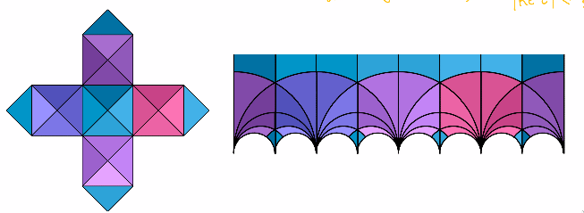
The dodecahedron and icosahedron correspond to the following:
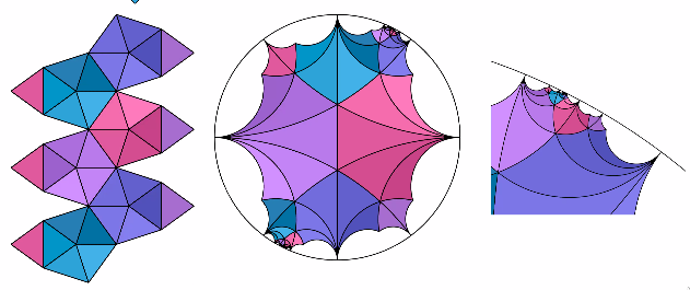
The cusps correspond to points of -fold symmetry, and correspond to , and the points converging to are given by ratios of Fibonacci numbers.
Remark 1.2.17.
Instead of just considering the icosahedron, we should consider an infinite strip with the given pattern in the picture.
1.3 Jordan Decomposition
Let . Then for all , we can decompose into Jordan blocks. In particular, we can write , where is semisimple and is strictly upper triangular (in some basis). The analogous decomposition for is . Now if is invariant under , it is invariant under both .
Consider the regular representation of on .
Lemma 1.3.1.
For any , we have .
Corollary 1.3.2.
If is an algebraic group, then for all . Moreover, if is a homomorphism, then and .
Proof.
By Chevalley, is the stabilizer of a subspace on and therefore because stabilizes the subspace, so do .
For the second part, we can pull back and then the desired result is obvious. □
1.4 More Solvable Lie Algebras
We will return to solvable Lie algebras. Assume .
Theorem 1.4.1.
Let be a Lie subalgebra. Then is solvable if and only if for all .
Proof.
One direction is clear by Borel. Here, is contained in the subalgebra of upper-triangular matrices. In the other direction, the form . In particular, we see that if , then this becomes a bi-invariant -form on . This gives a class in . Now we have an exact sequence
and here the unipotent radical is homeomorphic to , while is a product of simple nonabelian and a torus up to a finite cover. Then is the number of simple nonabelians, and so the morphisms generate .
Now suppose that . Now we will show that is solvable. It suffices to show that is nilpotent. By Engel, it suffices to show that any is nilpotent. Consider the subalgebra
This is the Lie algebra of an algebraic group
But then for all . Now if , then we have
so if , then . Now considering , we will obtain some condition on . These will have the same eigenvectors as . If is an eigenvector of with eigenvalue , then it has eigenvalue under . If there exists such that , then and thus .
Now if is linear over , then and . Next we see that because we can embed and then take . Then we see that , and then we see that all . Alternatively, if , then there exists a nonzero , but then . □
Definition 1.4.2.
Define the Killing form by
Remark 1.4.3.
Killing apparently lived a very sad life and did not get the recognition he deserved. Unfortunately, Andrei (and I) do not know more about him.
Theorem 1.4.4.
A Lie algebra is solvable if and only if .
Proof.
Consider the exact sequence
Then solvability of is equivalent to solvability of . □
Theorem 1.4.5 (Cartan Criterion).
A Lie algebra is semisimple if and only if the Killing form is nondegenerate.
Proof.
Suppose is degenerate. Then is a solvable ideal in . But then if is a solvable ideal with , then is an abelian ideal. Therefore, for all , we see that
and therefore for all , we have , so , and thus . But then . □
Corollary 1.4.6.
If is semisimple, then is a sum of simple nonabelians.
Proof.
Suppose is an ideal. Then (because it is a solvable ideal). Note that if is an ideal, then . □
2 Geometric and topological aspects
2.1 Lie algebra cohomology
There are three kinds of properties:
- •
General abstract properties;
- •
Properties derived from the structure theory ;
- •
Properties derived from the calssification of root systems.
We will begin with the first. If is semisimple, then:
- 1.
The category is semisimple. In particular, every finite-dimension -module has the form , where the are simple.
- 2.
The algebra has no deformations.
- 3.
All derivations of are inner derivations. In particular, we see that . In addition, in the exact sequence
the two outside terms vanish.
- 4.
For any Lie algebra , we have
and this exact sequence splits into .
All of these pheonomena fit under the umbrella of the vanishing of some cohomology groups.
Definition 2.1.1.
Let be a Lie algebra over a field and be a -module. We may consider the complex
and define
In the homework, we will show that , so we may define the Lie algebra cohomology .
For an example in low dimension, we see that is given by , so . For a more modern definition, we see that are the derived functors of .
We may motivate this formula in the following way from the de Rham differential. Suppose acts on a manifold . This gives a morphism into the vector fields. Then if are vector fields on and is an -form on , we have
Proposition 2.1.2.
The formula for is the same formula as in Lie algebra cohomology, where is the Lie derivative of along .
Proof.
Andrei’s proof is way too confusing. This is also Proposition 12.19 in Lee’s smooth manifolds book. The proof there is the same, but is done in a much easier-to-digest way. □
Theorem 2.1.3.
Let be a semisimple Lie algebra over a field of characteristic .
- 1.
If is irreducible and nontrivial, then .
- 2.
is the free anticommutative algebra on finitely many generators of degree contained in . When , this is the same as . This is also the same as the cohomology of the maximal compact subgroup. For example,
In particular, if is semisimple, then vanish for all . Also, we have an isomorphism , and this is just the space of invariant bilinar forms.
Proof.
- 1.
Suppose is nontrivial and irreducible. Without loss of generality, assume is simple and consider . We will show that multiplication by is homotopic to . Consider the form , which is nondegenerate. Then if are dual bases of , the Casimir element commutes with and is nonzero because . Now we will define our homotopy by
Now, we compute . We have
Then writing
we have
Now we may verify that all of the relevant terms cancel, so
The second term is given by inserting the tensor . But then is an invariant tensor, so .
- 2.
We may assume that or , so let be a connected compact Lie group. We will see that . We will compute ordinary cohomology using the de Rham complex. First, we will note that acts trivially on . To see this, observe that acts on forms by the Lie derivative , and if by the Cartan formula.
Now for any compact group acting on a manifold , the inclusion induces an isomorphism on cohomology. To see this, we simply note that is cohomologous to . Therefore, we may consider right-invariant forms in . But then
and the differential on is the differential from Lie algebra cohomology. Now if we consider , the differential vanishes. To see this, the map perserves the biinvariants but acts by on , and so , so . Because acts trivially on cohomology, it is also possible to see that
is a quasi-isomorphism. □
Example 2.1.4.
- 1.
Let be abelian. Then
- 2.
The condition that is compact is important. Note that
Next, we will actually prove that . In particular, by a theorem of Hopf, this is a Hopf algebra. Similarly, if is a compact Lie group then is a Hopf algebra. Here are some properties of the cohomology:
- •
It is graded and supercommutative.
- •
Under the map given by , if we write
then because .
Theorem 2.1.5 (Hopf).
Any finitely generated graded supercommutative Hopf algebra and the second property has the form .
Corollary 2.1.6.
If, additionally, our Hopf algebra is assumed to be finite-dimensional, then all of the are odd.
Proof.
Let be generators with . Then let be the algebra generated by . Then we know that , so each is a sub-bialgebra. Now it suffices to show that .
Suppose there is a relation of degree . But now if we consider the ideal modulo , which does not contain for grading reasons, then we have
and this must be a relation of smaller degree. Therefore we have no relations beyond supercommutativity. □
Now an interesting problem is to compute the degrees of the generators. For example, we have
Theorem 2.1.7 (Cartier-Kostant-Gabriel-…).
If is a supercommutative Hopf algebra over a field of characteristic , then
where is a (typically finite) group and is a Lie superalgebra over .
The elements with are called grouplike, and the elements with are called primitive. The grouplike elements give us , and the primitive elements give us .
Now we may take the dual Hopf algebra, and this gives us another graded supercommutative Hopf algebra. These give us algebraic supergroups over . But this algebraic supergroup must be an odd vector space. Another consequence of the theorem is that a commutative Hopf algebra over has no nilpotent elements. This implies that all group schemes over are reduced and therefore smooth.
Recall that if is a compact connected Lie group, then .
Theorem 2.1.8.
We have , where is the dimension of the maximal torus.
We would also like to compute the . In fact, are the degrees of the generators of . We know that every element of is conjugate to an element of . The normalizer of this is the Weyl group . Now, by definition, we have
and this is free on some generators of degree for .
Theorem 2.1.9.
The defined in the various ways are the same numbers and are called exponents of .
Example 2.1.10.
For , we have and . Alternatively, we can use the coefficients of the characteristic polynomial. In addition, we see that
and is generated by , and in general
In this formula, we observe that must be odd.
Proof of Theorem 3.2.8.
Use the Molien series. We have
Setting , we see that
This now gives us
by change of variables. □
2.2 Classifying Spaces and Flag Varieties
We already know that . On the other hand, we know the cohomology of the flag manifold is all even, and finally we have the cohomology
On the other hand, we have
For , this becomes the space of polynomials divided by symmetric polynomials of positive degree and has dimension . This is the fiber over of the map . To define , consider the category of spaces with a free action of (equivalently principal -bundles) for any group . Given a commutative diagram
with , we would like to consider the possibilities for for a fixed . If we consider the graph of , this is just a section of because acts freely, this is the same as a section of .
Theorem 2.2.1.
If is contractible, then there exists a unique compatible with .
Proposition 2.2.2.
For any compact group , there exists a contractible space with a free -action.
Corollary 2.2.3.
- 1.
is unique up to homotopy.
- 2.
is functorial in .
- 3.
For any free action of on , the map is the pullback of
for some map . Therefore, we see that
Proof of proposition.
For all compact, there exists an embedding , so it suffices to consider . Consider the embedding for some . For example, we have the action of on , so we can consider , which is contractible. Therefore we have .
In general, we can consider the action of on
and this last space becomes contractible as . To see this, it sits inside of , and thus as , we obtain a contractible subspace of . Finally, we have . □
Therefore, we have a tautological -bundle on and a tautological -bundle where the fiber above a subspace is the subspace itself. The vector bundle is the associated bundle of the -bundle and the -bundle is the bundle of unitary operators on the vector bundle. Also, we have proved that
The same statement holds for , real vector bundles, and the real Grassmannian. Explicitly over , consider the exact sequence
Now the kernel defines a map . Taking , we obtain the desired result.
Remark 2.2.4.
The spaces and are naturally approximated by algebraic varieties such as and are therefore ind-schemes.
We want to show that is contractible. We can consider the function on given by . Then are never collinear for and thus is homotopic to the identity. But then is never collinear to and therefore is nullhomotopic. We also see that is contractible. Also, is contractible and so are Stiefel manifolds
The Stiefel manifold has a free action of , so this is . We also see that . We know that the maximal compact subgroup of is homotopy equivalent to , so .
Remark 2.2.5.
The high-brow way that we prove that all of these spaces are contractible is by proving that they are weakly contractible, and then smashing the remaining part that weakly contractible implies contractible for spaces with the homotopy type of a CW complex.
Now the cohomology is intimately connected to characteristic classes for principal -bundles. If acts on a manifold , we have a map , so we may consider the Lie derivative for . For the Lie derivatives, recall the identity . This gives us a super Lie algebra with , , and . This gives us the super-Lie bracket
Now we see that , is given by the Cartan formula, and is the adjoint action of on itself. Therefore, if is a manifold with a -action, then is a supercommutative DG algebra with an action of .
If the action of is free, we may choose a -invariant metric on . For every , we have its projection onto . This gives us a connection, which is a -invariant -form with values in and thus gives us a map
Therefore, if a map , where is a supercommutative DG algebra means that acts on , we would like to give an interpretation of a connection such that .
Theorem 2.2.6.
There exists a unique acyclic supercommutative DG algebra with . We will denote this universal algebra by .
Proof.
Set and with acting by the coadjoint action. We set to be the zero map. We also set . Because must be an isomorphism, we see that with the coadjoint action of . Then we define by
Note that looks like , which are polynomials in multiplied by . For and , we can define . Therefore, is a derivation, and the Laplacian
is the identity on and . This implies that multiplication by on is homotopic to the identity and thus .
Now we return to our manifold and base . Then the image of are the so-called basic forms, which vanish on (horizontal) and are -invariant. In particular, they are killed by both . Then the map has kernel the horizontal forms, so we need to consider the horizontal forms.
Proposition 2.2.7.
Horizontal forms are generated by curvatures, which have the form
where is the map given by the transpose of the Lie bracket.
We now have
because . Therefore we can write
Therefore, we have and with zero differential, so we have . Now we have a transgression1 map , which is the “inverse” of the differential. This vanishes on .
Corollary 2.2.8.
. This is because is a perfect pairing.
In some sense, we have proven that
Theorem 2.2.9.
.
However, we would like to discuss . Now we want to describe the transgression. If , then want to compute , and then we can restrict this to by killing the horizontal forms. Therefore, polynomial functions on map to polynomial differential forms on by . This gives us something like
and this takes polynomials of degree to elements of degree . Now in the chain
the choice of does not matter. Also, this map is zero on because if , which is killed by transgression. Therefore, primitive elements of map isomorphically onto primitive elements of . Now we have explained the relationship between and .
We now want to add the third vertex of the triangle, which is . Recall that any element of is conjugate to some element of and that , which is a free algebra. Therefore,
We will see that this is free over .
Example 2.2.10.
For and , we have and , and also .
Now we have a map because the image of the map is a point, so we have to kill all positive degree elements in .
Theorem 2.2.11 (Chevalley-Sheppard-Tod).
Let be finite. Then the following are equivalent:
- 1.
is generated by complex reflections such that .
- 2.
is free over the invariants .
- 3.
.
There is a classification of all such groups generated by complex reflections, but Andrei does not remember what it is.
The key to the proof of this theorem is divided difference operators: If is a reflection, then is a hyperplane, so for all , we may consider . This vanishes on , lowers the degree by , and commutes with . For example, we could choose
Proof.
Let be a basis of . We will show that it is also a basis of over . Suppose there exists a relation , where . Then either or . Inducting on the degree of , if , then
Averaging over , we obtain the desired expression. If , then we can apply divided difference operators to reduce the degree. The divided differences of some function all vanish only when for all , which is equivalent to . Therefore we can assume , so if , then
form another basis of . But now we obtain a shorter relation
Therefore we have proved freeness. Finally, we see that the rank of over is .
Now note that is flat. Therefore is smooth. Recall that if is a scheme, a point is smooth if and only if a minimal resolution of is finite.2. The most important point to check is . Here, have a finite resolution
so after tensoring with , flatness gives us finiteness for .
To prove the final leg, we will use Molien series. Recall that is a cone with vertex and is also smooth, so it must be affine space. Recall that , where . Then
This implies that the number of generators is . This implies that . For example, if , then , and the exponents are . The next term in the expansion gives us the subgroup of all reflections fixing in , and in fact it is cyclic and contained in the roots of unity. Denote a generator by . Then we have
This implies that . For example, for , we have . Now set be the subgroup generated by reflections. Then , where has degree and has degree . If we order and , then because otherwise the would be algebraically dependent. Thus and in in fact the inequality is strict unless for all . However, both sums count reflections, which is the same for , so in fact . This implies that , and thus , so . □
Now we have a diagram
which commutes. In particular, is the regular representation of the Weyl group, which follows from the Lefschetz fixed point formula, which states that if , then we have
which says that the number of fixed points with multiplicity is equal to the intersection product of and . In our case, has no fixed points and thus its trace vanishes. For , all points are fixed, so we obtain .
Now recall that . Then maps to a -invarint -form that restricts to at the origin and that is the regular representation of . But then we see that and thus . This also follows from the fact that the composition maps to a point. Therefore we have a map
Both spaces have dimension , but we want to know if this is an isomorphism. Equivalently, we want to know whether the cohomology of is generated by . Both of these are -dimensional Gorenstein rings. Of course, we have for any closed manifold , and we call this the socle. This has dimension as a vector space. In addition, we have a perfect pairing
and in particular .
Another important example is a -dimensional complete intersection . This has
where is a regular sequence. For example, a dimension subscheme of the plane generated by a monomial ideal is Gorenstein if and only if it is generated by two elements. Equivalently, its Young diagram is a rectangle. Then the socle of is spanned by . In the case of a monomial ideal , this is spanned by . Now a map between Gorenstein rings is injective if and only if it preserves the socle. Then we know that , where is the rank, so . Therefore is a complete intersection. It has socle given by
and is the first anti-invariant . This means and thus the socle is the sign representation of . But then any with has to vanish along , so . In particular, . We conclude that the socle of is with
Now it suffices to check where goes in . We know that is the volume form on , so it goes to , as desired.
Remark 2.2.12.
There are other approaches to proving this result. Let and consider the locus
This is the zero locus of a section of , where are the tautological bundles. This has rank and thus . Now in , the class is given by the characteristic classes of . Like in Lefschetz, this acts by the identity operator on and thus is spanned by the characteristic classes of .
It remains to discuss the relationship between and . In principle, we can consider , but studying this requires spectral sequences. Alternatively, we will study this using the Weyl integration formula. Recall that the map
is generically -to-. Therefore we have a map
and because the action is free, the middle term is a smooth manifold. This gives us a map . This is a map between Gorenstein rings and is injective on the socle by inspection. Thus it remains to compute the dimension. By the Künneth formula, we have
The first term is the regular representation of and the second term is with the natural action. But then we see that has dimension . Chasing equivalences, we have
Here, all elements of have their degrees doubled. In particular, .
Remarks 2.2.13.
Recall that Lie algebra cohomology give the derived functors of . This is computed by resolving, taking invariants, and then taking the cohomology. This is a general principle in homological algebra, and in fact we can apply this to topological spaces. If acts freely on , then is nice (a smooth manifold) and therefore is nice. Otherwise, it is better to consider and the fibration . Then we can define the equivariant cohomology
and this is a module over . Then we can view (here the is taken as a superscheme) as a sheaf over . If acts on freely, then is homotopy equivalent to . The module structure over via . Now we obtain the skyscraper sheaf over with stalk at the origin.
In this language, we have , and this has a map to killing the positive degree part of the first factor of the tensor product. This recovers the cohomology of that we computed before.
Now let be a rank vector bundle on . Then is given by a map . This induces a map . Now there is a cell decomposition into Schubert cells, which is given by the row reduced echelon form of a matrix in . Now this gives a basis
where ranges over the Schubert cells. Then the character
is the character of an irreducible representation of . Now in terms of the characteristic classes, pulling back gives us classes , where are the elementary symmetric polynomials.
Now recall that parameterizes surjections , and if , then we know is a locus where a section of vanishes, and . Then . Thus if is a complex manifold, has rank , so is the locus where a vector field vanishes, so
Now parameterizes the locus where generic sections have rank , or equivalently . Therefore . Then describes the locus where sections have rank . Then the splitting principle tells us that we can write , where are the Chern roots. This is because if is an exact sequence, then .
Now we will consider the case of a line bundle . Then the curvature of is a class in . Then we can trivialize away from the zero locus of a section , If we draw a loop in the total space of over , then this may not be trivial. If the loop around trivial, then , but if there is a zero in the loop, then the integral is the total angle of rotation times the order of vanishing. Thus and .
Now if is the flag bundle of , then . Then
Now we can use this to prove that
To see this, note that every symmetric polynomial of degree is determined uniquely by its values on . It is enough to consider vector bundles , where is a sum of line bundles. Then if are sections of , then all must vanish, so .
Now we want to see that using equivariant cohomology. Consider the action of on . It is easy to see that the Schubert classes are preserved by the Borel subgroup. Now there is no difference if we take the Borel or the maximal torus , so we have a map
This is flat of length because we are taking the Chern roots up to permutation. If , then . Because while . Now if we consider the vector bundle
we see that . But then we must have for all and some .
By flatness, we obtain a result called equivariant formality. If , the fiber above is simply . If , then we obtain , and if is generic, then is a set of coordinate subspaces and is thus a disjoint union of points.
Now if , this has degree in and misses many fixed points. For example, on , the class hits everything, while the class misses anything with a in the first components. Thus we have a polynomial of degree in that vanishes on , so we obtain . Now we want a symmetric version of this, which is a Schur function in the
By an interpolation argument, this is exactly . In ordinary cohomology, we set and obtain the Schur function.
2.3 Minimizing norms
Let be a compact Lie group. This is associated to a complex Lie algebra . Then there exists a simply connected such that . By the Lie theorem, we have a central extension
Therefore complex representations of are the same as complex representations of . In particular, is linearly reductive.
On the other hand, by Peter-Weyl, has a dense subset given by , where ranges over all irreducible representations. This is a finitely generated commutative Hopf algebra generated by matrix elements of a faithful representation. Therefore it is for some linear algebraic group with . This also works when is not connected. For example, if is abelian, then .
Now we will prove that if is a complex reductive group, there exists a compact such that . In other words, every complex reductive group is a complexification of a compact Lie group. Now if is a complex reductive group, then there exists an exact sequence
Then is open in , and thus everything is algebraic. Therefore we have an embedding . Now all of the maximal compact subgroups are conjugate because any compact group preserves some Hermitian metric, so we hope for .
What we want to do is to minimize some norm. Consider . This is a finitely generated algebra with a linear action of , so if we take a -invariant subspace that contains the generators, then there is a closed embedding into a finite-dimensional -module as a closed orbit. Now choose a -invariant norm on and minimize it on . Set
Proposition 2.3.1.
.
Assuming this, choose , where . Then
and therefore . In fact, the real dimension of a compact subgroup is at most the complex dimension of , and in fact any compact subgroup is totally real in . Here a submanifold of a complex manifold is totally real if for all . In particular, we have and . Therefore it remains to prove the inequality.
First, note that is a plurisubharmonic or -convex function.
Definition 2.3.2.
Let be a complex manifold and be a real function. Then is plurisubharmonic if is positive semidefinite and strictly plurisubharmonic if is positive definite.
This is equivalent to the function being subharmonic for all open , which is equivalent to the Laplacian being nonnegative (or strictly positive). To see this, note that
and so we have the product of the Hessian and the norm of . Therefore the restriction of a plurisubharmonic function to a complex submanifold remains plurisubharmonic. Thus is clearly plurisubharmonic because its Hessian is the standard Hermitian metric.
Proposition 2.3.3.
The minima of any strictly plurisubharmonic function are totally real.
Proof.
Note that is in the kernel of the Hessian of . Therefore it cannot contain any complex lines and is thus totally real. □
There are some variations. Let be an affine variety (or a Stein manifold) and consider for some fixed . This is a Morse function for generic . Then the negative index of at any critical point is at most , so the tangent space contains no complex lines. This implies that has the homotopy type of a CW complex of real dimension at most . This can be found in a 1959 paper of Andreoti and Frankel about the Lefschetz hyperplane theorem.
Theorem 2.3.4 (Lefschetz hyperplane theorem).
Let be a smooth projective manifold of dimension . Let be a hyperplane section. Then the restriction map is an isomorphism for and injective for .
Now let be a complex reductive group and let be a representation. Then we know that parameterizes closed -orbits. For example, under the action of on by , the closed orbits have the form and the origin. Here, the only closed orbit in is the origin. Therefore, we have . For any closed orbit we can look for minima of a -invariant Hermitian metric , where is a compact real form of . We may assume that has the form . We would like to prove the following result:
Theorem 2.3.5 (Kempf-Ness; Matsushita-Onishchik).
The orbit is closed if and only attains a minimum. When this is the case, the minima form a single -orbit and there are no other critical points of . Finally, the stabilizer of is reductive.3
Corollary 2.3.6.
We can identify with the quotient of the critical loci of by . Equivalently, the moment map vanishes.
Returning to our example, the critical locus of is the set , which is the union of two lines. This intersects each orbit exactly once, as desired.
It is clear that if the orbit is closed, the minimum of the norm function is attained. Now we will assume Kempf-Ness and prove Matsushita-Onishchik. Write for the locus where the minimum of the norm is attained. Then we know that , where is the stabilizer of a point . However, we can extend this to the inequality
This implies that . Of course is totally real, so the reverse inequality holds and thus is the complexification of , so it is reductive. In fact, all inequalities are equalities, so is the dimension of any -orbit contained in . This implies that is smooth. We will also see later that is connected, so it forms a single orbit.
Now for , write . This is some Hermitian metric, so can be identified with the space of Hermitian metrics on . Then we know that
Recall that for reductive, there exists some metric such that is a compact real form . Then we have a morphism , and the image is . Then we know every element of is conjugate to an element of for a maximal torus , Therefore we can represent as for some , where . In particular, we have the decomposition . In our previous example, .
This means we can write , and only changes . Now if , we know
and therefore we can write
This is a convex nonnegative function. When the are not all of the same sign, we have a unique maximum, but not necessarily when all . We can consider the weights of the -action on in the characters of . In the first case, the Newton polytope contains the origin, so our function is strictly convex and bounded below. In the second case, the Newton polytope does not contain the origin, so the closure of contains some other vector and thus is not closed. This implies is not closed. There is a third case in which is contained on the boundary on the Newton polytope. In this case, we have a semistable point.
In conclusion, of has a local minimum, then the orbit is closed and there are no other critical points. In addition, for any maximal torus , the Newton polytope of the weights of the -action on contains the origin. This is called the Hilbert-Mumford criterion.4
Now consider the action of on coadjoint orbits in . Then every defines a function which is the Hamiltonian for the vector field . Recall that the coadjoint orbits are Poisson manifolds. For a basic example of a Hamiltonian, the function gives us the flow which is rotation with velocity . Changing coordinatse, we see that generates and generates . If we write , then . Of course, we have and thus
We obtain the same formula when is a larger diagonal matrix, where . In this case, we have
This implies that critical points of are the same as the zeroes of the moment map.
Now we can generalize this in several directions:
- 1.
We can consider GIT quotients. For example, if we have a character , then we can replace by
Instead of , we can consider .
- 2.
Many moduli problems are fomally quotients by infinite-dimensional groups. Then the moment map equations (or minimization of ) are very useful and important PDEs. A very classical example of this is the work of Hitchin-Kobayashi-Donaldson-Uhlenbeck-Yau-…who studied stable holomorphic vector bundles. In fact, stable holomorphic bundles are precisely those with Hermitian Yang-Mills connection. These minimize .
For example, if we consider a curve and a line bundle of degree , this line bundle lives in . Then we are looking for flat unitary line bundles, which have the form under a map . Therefore our line bundles are parameterized by
In fact, this is isomorphic to the Jacobian as a smooth manifold. More recently, there is the work of Chen-Donaldson-Sun in higher dimension.
2.4 Symmetric spaces
Now let be a complex semisimple group and be a maximal compact. Then is fixed under , which is an antiholomorphic automorphism of . Now consider a orbit of , which is thet set of positive self-adjoint elements of . Now . Also, has a -invariant metric, and this is unique up to multiple if is simple. Also, preserves the metric, so it acts as an isometry of , which is a symmetry about .
Definition 2.4.1.
Let be a Riemannian manifold. We say is a Riemannian symmetric space if for all , there exists some isometry fixing such that acts by on .
In particular, is an example of a Riemannian symmetric space. There is a structure theory of Riemannian symmetric spaces, and the classification is essentially the classification of all real Lie groups. Here are some properties of symmetric spaces. If lie on a geodesic, then is translation by the distance between . In particular, is complete. In addition, the isometry group of acts transitively on .
This implies that where is the stabilizer of some point . In particular, is compact because it is a closed subgroup of . We also know that commutes with , so is an inner automorphism. Now we have
where are transformations in and moves . We see that is the eigenspace and is the eigenspace. Therefore a Riemannian symmetric space is the same as a Lie group with a choice of automorphism and compact subgroup , where .
Now consider the symmetric space . If we choose , the involution fixing the north pole is the map
which has two fixed points. This means that does not have to have a unique fixed point. Now if we conjugate by , then the fixed locus is
Now if we take , we can remove the if we take . Now the classification of Riemannian symmetric spaces is as follows:
- 1.
Spaces of the form , where is a real Lie group and is a maximal compact group. These have negative curvature.
- 2.
Spaces of the form , where is a compact Lie group. Thus we have with the action of by conjugation.
- 3.
There are compact summetric spaces with positive curvature, and these are dual to the negative curvature case.
An important example of a symmetric space is the hyperbolic space . This is dual to . The classification reduces again to the classification of root systems, which sit inside the class of finite reflection groups. Of course, finite reflection groups sit inside discrete reflection groups. In fact, the maximal symmetric spaces have , and these are classified by
We also must have and because is the positive eigenspace of some involution and is the negative eigenspace. This gives us an -equivariant map . These are both irreducible and isomorphic, so these are multiplication by a real constant . If , then and . If , then and , and if , then and .
3 Semisimple Lie algebras
3.1 Reflection groups and root systems
Now we want to consider discrete isometry groups where is one of . This is in fact equivalent to the fact that for all , is discrete. Therefore the subsets are also discrete in . To see this, consider any point . Then the distance . Thus if is not discrete, the distances accumulate. If is generated by reflections, then the set of reflecting hyperplanes is discrete.
Now we will consider the Dirichlet fundamental domain
This is a locally finite intersection of half-spaces. We are mainly interested in the case where is compact, so we will have a globally finite intersection. In the compact case, we may have to subdivide the boundaries such that each facet corresponds to a particular :
In the globally finite case, we obtain . These generate and the relations are as follows: Note that is a facet of . It is also easy to see that . In the case of a reflection group, then and . In other words, is a symmetric set of generators. We also have more complicated relations coming from codimension strata. If the fixed hyperplanes of have angle , then is rotation by , so we obtain the relation . In fact, if we have the square lattice, then .
Theorem 3.1.1.
The relations above are all relations between the . This means that
Proof.
Consider the exact sequence . Now consider
But now we have a covering
However, is -connected, so this covering is an isomorphism. □
Therefore it remains to classify possible . First, however, we will consider a very classical example.
Example 3.1.2.
Consider a triangle with angles . Then we can consider the discrete reflection group . We have the following cases for where the triangle lives:
Thus in the first case is finite, in the second case it has polynomial growth, and in the final case it has exponential growth. To define the growth, we need to consider the length function on . Here, we count the number of hyperplanes separating , and this is the length , which is also the length of the shortest . Some nice properties are that and that . Then we consider the function that takes to the number of words with length less than , and consider the growth of this function.
There are finitely many solutions to , and these correspond to platonic solids (spherical) or regular tesselations of the plane (Euclidean).
Now we are ready to classify discrete reflection groups acting on or . We can embed , so the two cases are really the same. We want to impose that the normal vectors to the bounding hyperplanes span . We also assume that there is no partition of the normal vectors into two mutually perpendicular sets. We will carry out the classification using the connection to complex semisimple Lie algebras (or compact semisimple real Lie algebras). Consider the outer normals and consider the Coxeter matrix . Now we know
Because this is a Gram matrix, it is positive semidefinite. Also, the diagonal emenets are all positive and all off-diagonal elements are nonpositive.
Lemma 3.1.3.
Together with indecomposability, the two properties imply that either the are linearly independent (in which case is a cone over a tetrahedron, which is the image of under a linear map) or that , where has all positive coordinates.
In the first case, is the cone over a simplex and is finite. In the second case, is a simplex, so it is the image of . In this case, we obtain an irreducible reflection group in .
Proof.
Consider the matrix as a quadratic form. Then the kernal . For , denote . Thus . Thus if , we also have . Now suppose that some and . Then . If there exist such that , then . This is impossible if is indecomposable, so no can vanish for . Thus . Moreover, the kernel is closed under , so it must be spanned by a vector with . □
This implies that the classification of reflection groups in is the same as the classification of indecomposable positive-semidefinite Coxeter matrices. This is explicit and fun, and involves solving inequalities.
Now let for a compact group with maximal torus . Then write and . Then we have a decomposition
and we know is -dimensional if and only if is a root. Next, consider . Then we write , and this is unique. Then we have and and . Therefore we have an embedding , so an . Next, consider the map
We need so that is in the lattice spanned by the roots. The reflections in the roots generate a finite group of reflections, which also preserves the root lattice. Now we may consider the Cartan matrix . This is an integer matrix with on the diagonal and nonpositive off diagonal entries. The Cartan matrix must be positive definite.
Now each reflecting hyperplane is the zero set of a linear function (which is a root). Now we can choose a fundamental domain, and this gives us a partition of roots into positive and negative roots. After reflection by some , if is a positive root, then is still positive after . Therefore every positive root has a sum of the form , where the are the simple positive roots (corresponding the the faces). Moreover, this expression is unique (because the simple roots are independent as affine linear functions).
Now recall that for a semisimple Lie algebra , we have
where ranges over the roots. We know that , that , that , and that if . Also, there exist such that . If we write , then . Now our goal is go from root systems to Lie algebras.
Because every root is either positive or negative, and every positive root can be written uniquely as a sum of simple roots, we can write
Note that if is finite-dimensional, then is nilpotent.
Proposition 3.1.4.
The nilpotent Lie algebra is generated by , where are the simple positive roots.
Proof.
We show that if is a root, then . Consider the action of on . Now each is one-dimensional. Now recall that the weights of irreducible representations with respect to are . But now recall that decreases the weight by and increases the weight by , and so the action of is nonzero, as desired. □
Corollary 3.1.5.
The Lie algebra , where , where the are the simple roots.
The relations are given by
We will write . We also have and .
Lemma 3.1.6 (Chevalley-Serre).
For all , we have .
For example, for the root system with Cartan matrix , we have .
Proof.
Write . We will prove that if , then is invariant under . Then is a lowest weight vector, so would be a proper submodule, contracticting the simplicity of .
Now we need to prove that . This is clear for , so we need to check it for and . For , we have weights for (by the action of on ), so corresponds to the weight , so we must have (because otherwise it would generate an infinite-dimensional module). Now we consider the case when . Here, we have
Now if , we see and if , we also have vanishing. □
Theorem 3.1.7.
For a simple Lie algebra , we have with the Cartan matrix . Moreover, for any matrix such that , , and is symmetrizable, then the matrix is simple and finite-dimensional if and only if corresponds to a finite root system.
Remark 3.1.8.
Note that the conditions that , and is symmetrizable can be relaxed in principle.
3.2 Kac-Moody Lie algebras
Let be a matrix such that , and if and only if . Note this is weaker than being symmetrizable. Now we define the Lie algebra
Now we have the decomposition , where is the free Lie algebra generalized by the , whose universal enveloping algebra is a free associative algebra. Note if , then . Also, we have
so in fact all roots are already either positive or negative. Here, note that
and we also know that
The previous argument for shows that it is a lowest weight vector in . Now we know that . More generally, we can consider the maximal submodule of (which cannot contain the ).
Definition 3.2.1.
We define the Kac-Moody algebra to be the quotient of by the maximal submodules in and .
Theorem 3.2.2 (Gabber-Kac).
If is symmetrizable, then the maximal submodules in are generated by the Chevalley-Serre relations.
Theorem 3.2.3.
If , then corresponds to a finite reflection group.
Remark 3.2.4.
There are even larger generalizations of this, for example Borcherds-Kac-Moody Lie algebras and other classes of Lie algebras.
Now Chevalley-Serre tells us that for large enough , applied to any generator vanishes. Thus for any , there exists such that . I particular, any is contained in a finite-dimensional -module.
By definition, a -module is integrable if for all , the module decomposes as a sum of finite-dimensional modules. Thus, in this language, the adjoint representation of is integrable. Now we can integrate each -module to , and the matrix acts by reflection . Then we see that
and the generate the Weyl group of . In particular, it permutes the set of roots.
Recall that when we had an invariant quadratic form, we had the identity
Therefore there exists an invariant quadratic form if and only if there exists a diagonal such that is symmetric. Now note that , and are dual with respect to the quadratic form. In fact, we obtain expressions of the form
Now if we consider the ideal of relations , then we note that
Now note that any invariant bilinear form on is nondegenerate because is an ideal which does not intersect , and thus vanishes. If , then we can assume , and therefore we have a subalgebra , then for , is the lowest weight vector for with weight . If , then it is possible that the -module is finite-dimensional. Kac-Moody theory is about integrable modules. Also, recall that , and by Gabber-Kac this is the complete list of relations. Also recall the adjoint representation is integrable.
Example 3.2.5.
Consider . Note that if we want , we can only have . Now the three cases correspond to the Lie algebras . In the case where , or , then we need to enlarge to have . The extra elements in will be central, and we will need to consider a central extension of . Here, we will have
Now we have
These are called affine Lie algebras, and these correspond to reflection groups in . Now consider the case when . This is much more complex, and suppose , where . Then the quadratic form has signature . Now after we kill the Serre relations, we have our Weyl group , where
It is easy to see that . Now the vectors with form a hyperbola, and it is easy to see that are translations on the hyperbola. Note that these are solutions to and are units in . Also, note that
is periodic and the coefficients are .
The fact that there are no roots of in and the -action implies that there are no roots with . Now for , we would like to minimize the height . Now if , then we can decrease the height unless . Now in every -orbit of a root , either there is a simple root , so , or there is a root with for all . Now roots are either real (which means ) or imaginary (which implies exponential growth in the cone bounded by lines of slope ). In general, if the signature of our matrix , there is a similar picture, where we have a light cone (notation stolen from physics, all hyperboloids will asymptotically converge to this), and inside we have the funramental domain. Unfortunately, there is only a compact fundamental domain in low dimension, so the theory fails in high dimension. If the signature is worse, then the theory gets worse. However, every root is either real or belongs to the orbit of a fundamental domain (which is the set of vectors such that for all but finitely many roots).
It should be clear that if and only if . This explains why we end up with infinite-dimensional Lie algebras when we attempt classification.
3.3 Integrable representations of Kac-Moody Lie algebras
Let be a symmetrizable Kac-Moody Lie algebra and be the Cartan matrix. Then the Weyl group acts on .
Now if is a module and , by definition is a highest weight vector if for some and for all . Some examples of highest weight modules are Verma modules , which is the free module generated by a highest weight vector . Equivalently, we can write
This is not even close to being integrable (just note we can act infinitely many times by ). To make integrable, we need to be a nonnegative integer and . This gives us a candidate for an irreducible integrable module with highest weight1 . We will see later that this is indeed irreducible by the classification of irreducible finite-dimensional modules. We will also compute the character using the Weyl-Kac formula.
We will now consider the Casimir element. First suppose that and let be dual bases for the Killing form . Then the Casimir element is
Now because is dual to , we have
This acts by a scalar in because it commutes with all , and so
For any , we have . Now consider
Lemma 3.3.1.
For all , . In other words, .
Proof.
Note that permutes the set of positive roots distinct from . Therefore , and the desired result follows by splitting the expression for . □
Remark 3.3.2.
Some analog of this also makes sense if .
We can take any other function of the set , such as . Then the product
is a Laurent series in which is often analytically convergent. Under the action of , we obtain
Therefore this product is -anti-invariant. Note that the product is the character of acting on . Here, the operators have weight , and taking the sum, we obtain the expression. Therefore, the character of a Verma module is
Theorem 3.3.3 (Weyl-Kac).
The character of the integrable representation is given by
Returning to the Casimir element, we now write
For infinite-dimensional modules with highest weight, this expression makes sense because the final term in the sum is locally finite. Here, is the dual basis to the . This still commutes with the . Therefore acts on by .
To prove this, consider the exact sequence
Here, is some highest-weight module, so it has a surjection from . Thus there exists a resolution of by Verma modules of the form
By the action of the Casimir element, we have . In addition, the character of is -invariant by integrability. Together, we obtain that the character of is a sum of the form
where is either a sum of positive roots or zero, , , is anti-invariant under the action of by .
Lemma 3.3.4.
Every such that is a sum of roots can be brought by the action to the positive cone (where ). The positive cone is also called the dominant cone.
Proof.
Choose such that in the expression , is minimal. If , then we can apply and decrease . □
Lemma 3.3.5.
If , , and , then .
Proof of this result is left as an exercise to the reader.
As a consequence, we have:
- 1.
If , then the intersection of with the dominant cone is simply , and thus .
- 2.
In the exact sequence , the first term is simply . Now the cokernel is irreducible because it is integrable and therefore there is no room for other singular vectors. In fact, this can be continued to a Bernstein-Gelfand-Gelfand resolution of by
As a corollary of Weyl-Kac we obtain
Corollary 3.3.6 (Denominator identity).
Apply the formula to to obtain
and rearrange to obtain
For example, when , the positive roots are of the form , so . Then we have , and therefore we have
This has the more familiar form
For , this gives us the Jacobi triple product identity for theta functions
3.4 Affine Lie Algebras
Let be a group of isometries in . For example, if are reflections along the sides of an equilateral triangle, we have the group. Now isometries of embed in isometries of because we can embed as a horocycle. Now consider the group generated by with of infinite order. If we consider spheres in , we have an action of on which commutes with the action of on . Note that stabilizes a vector of negative norm. In the limit as the radius approaches , the curvature approaches , so we obtain .
Now the semidirect product stabilizes a null vector, so it acts on . Now if we fix that preserves the form , then if we consider the light cone where , then our isometry group acts in a way such that orbits are like parabolas. In the case of , the orbit of a single point in will lie on a parabola when we embed in .
Now our reflection group could have Cartan matrix or . The first corresponds to a central extension of while the second corresponds to a twisted loop algebra. Here, if is a Lie algebra and is an automorphism of order , then we may consider the subalgebra
For example, note that is generated by the matrices
Then . If we define , then for , is contained in the kernel of the map
Now note that if we set , then the Lie algebra is graded by . Because is degenerate, only one of these two gradings is internal. To restore the grading, we introduce the element , where and . Now we set
where we set . Now we have a map
Now because there are three simple roots, the matrix of the invariant bilinear form is
and this has signature . In the basis of , this takes the form
which is precisely of the form .
Now we would like to describe the central extension in terms of matrices. Here, we have
then we can write if we set . Using integration by parts, this is skew-symmetric. Now we have
Now the eigenvalues of on each factor are . The values are positive for . Now if we define
then if we set , we obtain
This is simply the genus theta function , which has the property that and that
Therefore is a section of a degree line bundle over . Note that converges analytically if . Because is invertible, we may use it as a clutching function. By Riemann-Roch, only has a single zero at .
Another way to write solutions of the equation is using the form . Here we want to think of as , so if we apply , we have
and thus we have . Therefore , and thus everything is unique up to a multiple section of a line bundle on . Classically, this is the Jacobi product formula. As a sum, we really have the sum in the Weyl-Kac formula, because
This also satisfies some -difference equation, so is a section of a Line bundle of . In general, we have
and this can be rewritten as an expression in the characters of is we sum over first and as a theta function if we sum over the lattice first.