Lie groups and representations I
Lie Groups and Representations
Fall 2020
Notes by Patrick Lei
Lectures by Andrei Okounkov
Columbia University
Disclaimer
These notes were taken during lecture using the vimtex package of the editor neovim. Any errors are mine and not the instructor’s. In addition, my notes are picture-free (but will include commutative diagrams) and are a mix of my mathematical style and that of the instructor. If you find any errors, please contact me at plei@math.columbia.edu.
1 Basic Notions
Definition 1.0.1.
A Lie group is a group that is also a manifold. Here, manifold could mean a smooth manifold, complex manifold, or many other options.
Example 1.0.2.
Locally, every Lie group looks like . An example of a complex Lie group is .
Remark 1.0.3.
If is a field with topology, then the additive or multiplicative group of are topological groups, but usually not Lie groups.
Example 1.0.4.
Let be prime and consider the field of -adic numbers. This has a topology, but is not locally isomorphic to a vector space. Here, the base of neighborhoods of is formed by the fractional ideals , whereas neighborhoods of in are not subgroups.
Remark 1.0.5.
It is possible to develop analysis for the -adics and consider -adic Lie groups.
More generally, one can define a class of “manifolds” by postulating local models and the corresponding algebras of functions. For real manifolds, the local model is and the algebra is . Then a map is if and only if it pulls smooth functions back to smooth functions. To an inclusion , we will associate a “restriction” . This is known as a (pre)sheaf of algebras on . To be a sheaf means that given the restrictions
the first restriction is injective and its image is
To define complex manifolds, we consider the sheaf of holomorphic functions.
For some of the “other options,” we may consider algebraic varieties over a field , where the algebras of functions are reduced commutative algebras of the form . If we give up the idea of being reduced, we obtain schemes over . Algebraic varieties are both more flexible (singularities are allowed) and more rigid (any piece of the map determines the whole thing) than smooth manifolds.
Example 1.0.6.
Consider the group . is a Lie group of dimension for and , and in general, is the group of -points in the algebraic group defined by the equation .
In algebraic geometry, any variety contains an open set of smooth points. Because any group is a homogeneous space, all points must have the same properties, so they must all be smooth.
Definition 1.0.7.
A Lie group acts on a manifold if there is a map of manifolds such that and .
For all we can define the orbit and the stabilizer. If all of forms one orbit, we say is homogeneous or that the action is transitive.
Example 1.0.8.
Let . Then the action can be given by
- Left
-
;
- Right
-
;
- Adjoint
-
;
1.1 Examples of Lie Groups
For now, for real Lie groups, the notion of manifold we will use is that of a smooth manifold.
Example 1.1.1.
The additive group is a Lie group. In one dimension, the only connected manifolds are and .
Example 1.1.2.
Recall the classification of two-dimensional manifolds. First, any Lie group is orientable, so we will consider only the orientable manifolds. These are classified by their genus, and only the torus is a Lie group. To see this, note that Lie groups have a trivial tangent bundle. A global frame for is given by translating a basis of by . Therefore, we can write .
Remark 1.1.3.
By the Hopf index theorem, the self-intersection of inside is , so the index of a vector field on is .
We will now consider some -manifolds. In particular, is the Lie group . Note that unitary transformations of send to itself. Therefore, we can send one basis element anywhere, but if we insist that the determinant is , the second basis vector is sent to a unique target. Thus acts transitively on with trivial stabilizers. Alternatively, we can write
All connected real Lie groups, as manifolds, have the form
The maximal compact subgroup is a product of and simple nonabelian Lie groups. The simple nonabelian Lie groups are all built from in some sense.
Corollary 1.1.4.
The only finite-dimensional division algebras over are .
Note that acts on by rotations. Therefore we have a map with kernel , so we have an exact sequence
Heuristically, this means that left translation and right translation are as different as can possibly be.
Now we have seen groups like . In fact, the groups , the symplectic groups, and a few exceptional Lie groups, make up all simple compact nonabelian Lie groups (up to discrete centers).
1.2 Lie Group Actions on Manifolds
Recall the notions of action, orbit, stabilizer, etc. Then we have a map
that is equivariant, so the differential of this map has constant rank . Locally, the map looks like . Locally, the orbit looks like and the stabilizer looks like .
Theorem 1.2.1.
The stabilizer of any is a submanifold of . By definition, it can be upgraded to a Lie subgroup of . In addition, there is a neighborhood of such that is a submanifold in . If is compact, then is a submanifold.
Remark 1.2.2.
- 1.
need not be a submanifold of . The classical example is when acts on by flow along a vector field. For example, if , we can choose the vector field to be a constant vector field with irrational slope. The orbits are dense in . In fact, we obtain a group homomorphism with dense image.
- 2.
For algebraic actions, orbits are much nicer because for algebraic, contains a dense open subset of its closure and in fact is open in its closure (consider acting on ).
Let be a Lie group acting on a manifold . We will denote the stabilizer of as and the orbit of as . Note the orbit is not necessarily a submanifold., but is locally a submanifold. One such example is when acts on by time evolution according to some ODE. This type of behavior is studied in the field of dynamical systems.
Example 1.2.3.
A homomorphism is a special case of an action. If acts by left or right multiplication, we see that is a Lie subgroup of and may or may not be a Lie subgroup. We will call these “virtual Lie subgroups.”
Now we will discuss the space of orbits . Right now, this is still a set, but we can canonically make it a topological space with the quotient topology.
Remark 1.2.4.
This quotient space is very rarely Hausdorff, so in particular it is almost never a manifold. For example, if we consider acting on , we see that the quotient space consists of two points, where the point is closed and the point is a generic point.
Example 1.2.5.
Now consider actions acting on . Then there are several cases:
In these cases, the orbits look like this:
In the third case, the orbit space is . In the final case, even though the orbits are closed, the space is still not Hausdorff. In summary, may be non-Hausdorff in a very complicated way.
Note that has a natural sheaf of functions. If is open, then is open in , where is the projection. We will declare the functions on to be the -invariants. In the best case scenario, when is sufficiently small, we have where the action is contained entirely in the second factor. Therefore functions on defined in the new sense are the same as normal functions on .
However, there is no reason to expect this kind of behavior. We may get interesting behavior even for quotients by a finite group. For example, consider and let . Then is simply the closure of the upper half-plane with the negative and positive real axes glued together, so we obtain a cone with total angle . We see that is a manifold near every point except . At , we study functions of the form such that , which are functions of . It is easy to see that these satisfy the equation .
Similarly, if we consider acting on by roots of unity, then we will obtain invariants satisfying . This is known as the surface singularity.
Remark 1.2.6.
Note that is very different from because we take the second quotient in the category of complex manifolds. Here, and the projection is a double cover branched at . There is a similar result for .
More generally, we have the following result: a finite subgroup is generated by complex reflections if and only if . In general, is singular.
Example 1.2.7.
Consider the permutation group . Each transposition is a reflection in the hyperplane . Therefore the coordinates on are the elementary symmetric functions
for . This is an important notion in representation theory because we can consider the map
In general, can be replaced by the Weyl group.
In summary, may have complicated topology in singular. Complexity is good in math, but it is also good to have the simple cases. The best possible case is when the action is proper, i.e. that the map is proper (ensures the quotient is Hausdorff), and free, i.e. that there are no stabilizers.
Theorem 1.2.8.
Let be a free and proper action of a Lie group on a manifold . Then is a manifold and the projection is a locally trivial fibration with fiber .
Example 1.2.9.
Here are some examples of a free and proper action:
- 1.
The action of on . Then is an embedding and is in particular proper. Therefore is a manifold.
- 2.
Any free action of a compact Lie group.
Proposition 1.2.10.
The map is open.
Proof.
Note that is open. □
Note that the quotient by a group is a special case of a quotient by an equivalence relation.
Proposition 1.2.11.
Suppose is open and a quotient by a closed equivalent relation. Then is Hausdorff.
Proof.
Suppose that be such that such that . Then there exists a neighborhood of not intersecting , so there exist such that . These project to disjoint opens, so is Hausdorff. □
In our situation, is the image of . By definition, the action is proper if this map is proper.
Proposition 1.2.12.
Suppose is proper. Then the image of a closed set is closed.
Proof.
It suffices to prove is closed. Suppose . Then , which is compact. Thus we can find a subsequence , so because is continuous, . □
In particular, in a Hausdorff space, all points are closed. In terms of our group action, this means all orbits are closed.
Proof of Theorem 1.2.8.
Fix a point and look at the neighborhood of . Consider the differential of the action map . Because this map has maximal rank everywhere, if we choose coordinates along and along and for , the differential is simply .
Choose a submanifold transverse to the orbit, we can consider the action . We see that this map is a local diffeomorphism, so we need . This is not obvious and requires properness. One can imagine that there exists such that for any .
Choose a sequence that shrinks to . Then we consider the set . Then we can consider
with a fixed neighborhood of removed. This is compact by properness. If lies in the intersection of all such sets, it must stabilize , which is impossible. □
Remark 1.2.13.
For algebraic actions, it is possible that is free but for all open , for all . For an example, acts on cubic polynomials in . The generic polynomial has three roots and has stabilizer , but has trivial stabilizer.
Theorem 1.2.14.
Suppose the action of on is proper (but possibly not free). Then the normal bundle of is a vector space with an action of , so there exists a neighborhood of isomorphic to . This is a vector bundle over the orbit with an action of (it is precisely the associated bundle).
Now note that the stabilizer of is compact because the action is proper. We would like to find a -invariant slice at . To do this, we will need to discuss metrics. This is a smooth nondegenerate positive-definite quadratic form on each fiber. Then we can define the length of a curve by
There exist curves that minimize length locally, and these are called geodesics.
Then there is a map given by following a vector along the geodesic in the direction of for time . This is a local diffeomorphism and is closely related to the exponential for Lie groups. Later in the lecture, we will prove that if acts on and is compact, then has a -invariant Riemannian metric.
In particular, there is a -invariant Riemannian metric on . Then we can write . Identifying with the normal bundle , then the slice is simply .
Now consider the action . If , then by definition. Therefore, we can write
where acts by . This is -equivariant and locally an isomorphism.
Theorem 1.2.15.
This is an isomorphism of is a neighborhood of the orbit of . Note that we can scale any to the unit ball.
Corollary 1.2.16.
The neighborhood of the orbit of in looks like .
Corollary 1.2.17.
The stabilizer of any nearby point is conjugate to a subgroup of .
Remark 1.2.18.
Sometimes the quotient by the action is denoted by .
Corollary 1.2.19.
The manifold has a -invariant metric.
Proof.
Let . Then for a vector , we can associate and to , but these must have the same length because they differ by an element of the stabilizer. This gives an invariant metric in a neighborhood of the orbit. Finally, we can sum the local metrics over a partition of unity to obtain a global invariant metric. □
Theorem 1.2.20.
Let be a compact Lie group acting on a manifold . Then has an -invariant metric.
Proof.
Choose some Riemannian metric on . Then choose a Haar measure on and define
To show invariance, note that
More generally, suppose acts on an affine linear space by affine transforations and suppose there is a closed convex -invariant subset . Then there exists an -fixed point (by the same integration argument).
Now we will show existence of the Haar measure. Recall that by left translation. Then we may choose an -valued -form on , and this gives a finite volume form if the group is compact.
2 Classification of Lie Groups
2.1 Topology of Lie Groups
Recall that if acts on properly and freely then is a locally trivial fibration with fiber and is a manifold. Now suppose is a Lie subgroup of . Then acts freely and properly on . Therefore we have a map and is a manifold. Our goal is to use this fibration to understand the geometry of its ingredients.
Example 2.1.1.
Consider and let be the set of diagonal matrices in . Then to compute , note that acts on and hence on . The stabilizer of a point is , and thus is the Hopf fibration . An illustration of the Hopf fibration is below:
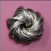
Any two fibers are linked as the Hopf link, so this is not a globally trivial fibration.
Example 2.1.2.
Consider acting on itself by conjugation. This fixes , so it acts by conjugation on . Because the norm of the matrix is preserved, we have a map with kernel the center of , which is just . By dimension arguments, the map is surjective, and thus we have realized .
We can discuss various topological invariants of Lie groups, in particular their homotopy, homology, and cohomology groups. We will begin with , the set of connected components. If is a Lie group, then is a group isomorphic to , where is the connected component of the identity. It is clear that under the natural map .
Example 2.1.3.
Let and let . Then any path connecting in descends to , so the kernel of is exactly the image of the transport .
Recall that we have a long exact sequence
arising from the fibration.
Theorem 2.1.4.
Let be a topological group. Then is abelian.
Proof.
The homotopy exhibits a homotopy between and for two loops based at the identity. □
Remark 2.1.5.
is not abelian. In fact it is equal to .
Let be a covering space. Then we have a map given by transport, and if , then is the universal cover.
Proposition 2.1.6.
If is a Lie group then so is its universal cover by multiplication .
Corollary 2.1.7.
If is a connected Lie group, then there exists a unique simply connected Lie group such that is an exact sequence.
Example 2.1.8.
The map is a universal covering. An even more basic example is the cover .
Proposition 2.1.9.
Suppose is a connected Lie group and is a discrete normal subgroup. Then .
Proof.
Let and consider the map . Because is connected, the image is a point, which must be because we can choose . □
In summary, any connected Lie group has the form , where is simply connected and is a discrete subgroup of the center.
Corollary 2.1.10.
If is abelian, then is of the form , where is some discrete subgroup, and this means that .
Remark 2.1.11.
This allows us to prove the fundamental theorem of algebra. If is a field extension, then is abelian and connected. Then for , this is , for this is , and for this is , which is impossible.
Here is a very important ideal in Lie theory: Consider a Lie group with identity . Then if we consider , we can reconstruct a lot of information about . An obvious limitation of this approach is that some Lie groups are locally isomorphic.
Example 2.1.12.
Recall that is a double cover of , so they are locally isomorphic. In particular, any group is locally isomorphic to , where is discrete.
Our strategy for dealing with this is to determine the universal cover, which is equivalent to determining . We will see later that simply-connected Lie groups are determined by the infinitesimal data.
Previously, we discussed the long exact sequence arising from a fibration. To make this precise, we need to define . But this is simply the group of homotopy classes of based maps from to . For , we can see that is commutative by the following picture (or the fact that is a double suspension).
Very often, is a sphere, with homotopy groups
Not much is known about the higher homotopy groups of spheres, and computing them is a central problem in modern algebraic topology. Fortunately, it is easier to compute the homotopy groups of Lie groups.
2.2 Lie Algebras
We will discuss reconstruction of simply-connected Lie groups from their local data. This can be phrased as an equivalence of categories. On one side, we have the category of simply-connected Lie groups, and on the other side, we have the category of Lie algebras. We will define a functor from Lie groups to Lie algebras that is an equivalence of categories.
We will define plus some extra data, and for any , we wil define .
Example 2.2.1.
Let be a Lie group homomorphism. Then we can differentiate to see that
This means that the morphism is determined by an ODE, and so it must be linear. Then is precisely the map between Lie algebras.
In general for , then we can differentiate with respect to at to obtain a system of first order ODEs. Then solvability of these ODEs is a condition on that is equivalent to being a homomorphism of Lie algebras.
Definition 2.2.2.
A Lie algebra is a vector space with a bilinear operation
such that that satisfies the Jacobi identity:
We will construct the Lie bracket out of multiplication in . If we simply differentiate the multiplication , the differential
is simply the addition. This is a linear map, but it tells us that all Lie groups are the same locally.
Therefore, we need to consider higher order terms in the Taylor expansion of . This is
and the quadratic term is a bilinear form with no quadratic terms in or . This is not independent of the coordinates because if we choose , then the multiplication becomes
In barticular, we have , which does not necessarily vanish. However, it is symmetric, so we can define the Lie bracket
In mathematics, there is a high road and a low road. The low road is to write everything in coordinates, which is sort of what we did here. It’s good to be able to take the low road, for example when we need to compute with a computer. A. Okounkov
Remark 2.2.3.
There are many other definitions of the Lie bracket.
- 1.
We can consider the commutator in . If we assume , then we have . The differential of the commutator vanishes, but the second differential is precisely the bracket.
We need to prove that the commutator satisfies the Jacobi identity, which can be restated as
Now define . Then the Jacobi identity says that is a derivation of the Lie bracket.
Note that if is a vector space with , then is an algebraic subgroup. If we apply the Lie functor, we see that
Consider the adjoint action of on itself. This fixes , so it gives a representation of on . If is a matrix group, then this is really a product . If we write this out in coordinates, we see that the adjoint representation of takes values in and thus when we differentiate. If we take the derivative , we obtain a map
We simply need to check that . But this is obvious because the left hand side comes from differentiating and the right hand side comes from differentiating .
Remark 2.2.4.
This gives yet another definition of the Lie bracket.
2.3 Correspondence between Lie groups and Lie algebras
Now let be a smooth manifold with an action of a Lie group . Then is an algebra that is acted on by . Then we know that is simply the space of vector fields. Then we can write , where is the ideal of functions that vanish at . For any derivation, . This defines a tangeng vector at any . In particular, defines vector fields on . Then we know that derivations form a Lie algebra.
For example, consider the action of on itself by left translation. Then we have a map . In addition, it is easy to see that this gives right-invariant vector fields on . On the other hand, right-invariant vector fields are determined by their value at , so we have an isomorphism of vector spaces. In fact, this can be upgraded to an isomorphism of Lie algebras.
Returning to the main point, we want to prove
Theorem 2.3.1.
The functor is an equivalence of categories.
Theorem 2.3.2.
Let be connected Lie groups with . Then any homomorphism is uniquely determined by .
Proof.
We know that . Then if we differentiate with respect to , then
This gives us a system of first order ODE. By connectedness, there is a unique solution with prescribed initial condition. □
Later, we will see that the mixed partials are equal (or the curvature vanishes) if and only if is a Lie algebra homomorphism.
Remark 2.3.3.
There is no homomorphism of Lie groups from corresponding to the identity homomorphism between the Lie algebras.
These ODE that we obtain from differentiating the multiplication naturally lead to the concepts of connections and curvature. Suppose we have a locally trivial fiber bundle over a base with fibers . Then the idea of a connection is to be able to lift paths downstairs to paths upstairs respecting concatenations of paths.
Fix a Lie group acting on the fiber . Then we say the structure group is contained in if all transition functions may be chosed to be in . For example, a vector bundle is a locally trivial bundle with structure group . We can use the same transition functions to glue copies of , and we obtain a principal bundle . Then the old bundle can be obtained using the associated bundle construction and a connection on a principal -bundle induces a connection on any associated bundle.
In our case, we are talking about the trivial -bundle over . Then sections are maps from to . In coordinates, these are lifts that are invariant under the action of on the right. This means we can consider the value at , which means we have a map . Thus a connection can be thought of as a right-invariant Lie algebra-valued -form. However, this is dependent on the trivialization. If we change the section by a function , we know a section is contant if
However, if we conjugate by , then we need to differentiate , and obtain
where .
Next, when does the transport along the path depend only on the endpoints? We can consider
- 1.
Small changes, i.e. homotopies with fixed endpoints. In this case, the connection is flat.
- 2.
Paths up to homotopy, i.e. .
Proposition 2.3.4.
A connection is flat if and only if its curvature is identically zero.
The curvature is a certain -form that measures the difference between two solutions to an ODE. If we transport along , then we obtain the commutator
Thus if the connection is flat, then the curvature vanishes. In the other direction, suppose we have two homotopic paths. Then if we break down the square into squares of size , then each square changes the result by , and so if we make small enough, the change vanishes.
Returning to our original problem, suppose we have a map . Then determines a connection on . On we have the canonical -form If is a Lie algebra homomorphism, then
and thus the curvature of the connection induced from is the differential of the curvature of , which is identically zero.
Remark 2.3.5.
All of this can be expressed in elementary terms. First, we have . Then we have
Thus we have proved the following theorem:
Theorem 2.3.6.
If is a simply connected Lie group and is a Lie algebra homomorphism, then there a unique map such that .
For example, if we want to prove that , we write
and note that the second term in the sum equals .
Recall the differential equations that we constructed for a homomorphism of Lie groups from the Lie algebra. These equations are right-invariant in both the source and the target and imply that is a homomorphism.
Example 2.3.7.
Here is a silly example: Note the isomorphism . Then and so we have
for some constant . In the other direction, we have , so
for some constant . The solution to the second equation is clearly the exponential function, and the solution to the first is
Invariance implies that is a homomorphism.
Theorem 2.3.8 (Lie).
For any simply connected Lie group , the map
is an isomorphism.
Here are some applications:
- 1.
Any connected abelian Lie group of dimension is of the form , where . Thus .
- 2.
Not all Lie groups are matrix Lie groups. However, every Lie algebra is a matrix Lie algebra in characteristic . In the category of Lie algebras, we can always lift the adjoint representation to the center of . However, when we consider the adjoint representation of as a Lie group, we cannot lift to the center.
For example, consider . This has . Then has in the center, and so any map
corresponds to a map of Lie algebras . This gives a map , which then lifts to a map . In particular, all linear representations of factor through are are thus trivial on the center.
Definition 2.3.9.
Suppose is a real Lie group with Lie algebra . Then if we take the complexification , this gives a map for the complex Lie group corresponding to . We say that is a complexification of and that is a real form of .
Remark 2.3.10.
Note that this relation is generally many-to-one. In particular, both and are real forms of .
Now let be a Lie group and . Then is a homomorphism of Lie algebras. Thus there exists a unique map
and this is the matrix exponential for matrix groups. Also, . In addition, if , then we can exponentiate in either order.
Theorem 2.3.11 (Lie).
For any Lie algebra over or , there exists a unique simply-connected Lie group with Lie algebra .
This gives a correspondence between our linear local data and nonlinear global data. We can construct manifolds either as:
- 1.
A quotient of something simpler. If is a simply-connected Lie group, then if we choose a point , then we can consider smooth paths from to . Then the tangent vector at time , and for a smooth homotopy between paths, If the curvature vanishes, then we have
Then we can write as the paths in the Lie algebra modulo solutions to the equation. Fortunately, the analysis reduces to first-order deformations.
- 2.
As a “submanifold” of something simpler. Write . Then we have a map with some kernel . Thus is the universal cover of . Therefore, at least locally, every element of the Lie group is a matrix.
A problem with this approach is that need not be a submanifold. If we have the map with dense image, we obtain a foliation, so individual leaves are (locally) submanifolds, but we do not globally obtain a submanifold. In particular, if is an injective Lie algebra homomorphism, we have a foliation with leaves corresponding to the cosets of in . In particular, we have the field of tangent planes . Thus the cosets may be reconstructed either as leaves of the foliation or as integral manifolds for this field of tangent -planes (a section of a bundle of Grassmannians over ).
Note that an integral manifold for a field of tangent -planes is a -dimensional manifold which is locally a submanifold such that is precisely the value of the field of -planes at every point . The idea to construct this in our situation is to start by finding an embedding . The main obstacle to this plan is that a field of -planes may not have any integral manifolds for .
A connection is a special case of a field of -planes. Here, a connection on a locally trivial bundle gives a field of tangent planes that are transverse to the fibers of . Then the existence of integral manifolds is equivalence to flatness. There is a classical criterion for the existence of integral manifolds.
Theorem 2.3.12 (Frobenius).
A field of tangent -planes in has integral manifolds if and only if for all the set of vector fields tangent to forms a Lie subalgebra of .
Proof.
Suppose we have integral manifolds . Then a vector field is tangent to the integral manifolds if and only if , which implies that .
Conversely, suppose that is our field of -planes. Then denote to be the set of vector fields tangent to . Then we have this following picture:
Thus we have
Here the first are arbitrary and the last are uniquely determined. In particular, we have a basis of the form
Then we see that
and so . This means that locally, the connection has curvature zero, and thus there are integral manifolds. □
Returning to our case, consider and consider the tangent field , where is a Lie subalgebra. Then
The right-hand factor is already closed under the commutator. By the Leibniz rule, we see that is also closed under and hence has integral manifolds.
Choosing the integral manifold that contains , this is a subgroup of . However, it is not a Lie subgroup in general. For any integral manifold and , then is also an integral manifold because the field was right invariant. If , then because is integral and contains , so for all , then . Hence is a connected Lie group. If is not -connected, then we can take the universal cover. Thus we have proved
Theorem 2.3.13 (Lie).
For any Lie algebra over , there exists a unique simply-connected Lie group with .
Remark 2.3.14.
When is algebraic? Not every Lie algebra over is a Lie algebra of an algebraic group. Most differential equations with algebraic coefficients do not have algebraic solutions.
For example, the irrational winding of the torus corresponds to .
3 Representations
Let be a group. Then a representation of over a field is a map . Here, we will take and strongly prefer . We will call a representation of a -module. These form an abelian category, which is not something we will dwell on too much. A map between two representations is an “intertwining operator” which is something that makes
commute. Then both are submodules. If has a nontrivial submodule, then it is reducible. Otherwise, we call it irreducible. If we have an exact sequence
then is a submodule of and is a quotient.
Definition 3.0.1.
A representation is called semisimple (or completely reducible), if , where is irreducible.
If are representations, then acts on by . This comes from the map .
We have a notion of characters that send a representation to the conjugation-invariant function . Then it is easy to see that and that . This is a semiring homomorphism, so we can form the representation ring . This is the -group of the category . Also, note that if
is exact, then we see that . Thus we can impose the relation .
At first sight, it seems that taking the character loses a lot of information. However, if we have all of the traces, this means we can compute all of the eigenvalues. Thus, we can reconstruct up to conjugation from its character.
Next, if is a -module, then also acts on by . Also, as a -module.
3.1 Finite Dimensional Representations
Consider the simplest groups we know: . First, all of these groups have the same finite-dimensional representations given by
and in the other direction, we can complexity to , and then is simply-connected. However, note that is not simply-connected, so we cannot use the same argument for . Also, representations of and are semisimple, but has the representation
which is a nontrivial representation in two dimensions that is not semisimple.
Second, we note that all representations are semisimple because is compact. To see this, note that is compact and thus every representation has an invariant Hermitian form (by averaging). Then for , we can write .
Then all irreducible representations of can be described as symmetric powers . This has basis , where . Here, the maximal torus acts by
We will find this structure in the representation of . We know has a basis
Then we see that
and . Also, note that . Then shifts the weight by and by .
Lemma 3.1.1.
If is an eigenvector of with eigenvalue , then and .
Proof.
Note that . A similar argument gives the result for . □
Classification of irreps of .
Let be irreducible and be an eigenvector of with eigenvalue . If , then replace by . The eigenvalue cannot grow forever, so eventually we reach such that and . This is called the highest weight vector.
Now we will show that is the span of . This is clearly invariant under by construction. Then note that
Because is a combination of by the commutation relations, we see that the span of is a subrepresentation, so it must be everything. Then because , then there exists a minimal such that . This implies that , but to show this, consider , which is a multiple of .
The rest of this proof is left as an exercise. □
Remark 3.1.2.
Representations of correspond to integers .
3.2 Harmonic Analysis on Compact Groups
Let be a compact Lie group and consider representations . We would like to do harmonic analysis on . Our prototype will be . If is the Haar measure, then we can write
as a Hilbert Space. Recall that a Hilbert space is a complete inner product space, and the inner product on is
We can write . Then recall that are precisely the irreducible representations of . Here, is the closure of the algebraic direct sum. Next, for any , we can take the Fourier transform
where . We will generalize this to an arbitrary compact group.
Our main issue is that for non-abelian groups, not all irreducible representations have dimension . However, we will have a correspondence
where is the Haar measure. These matrix elements of irreducible representations are in fact analytic. When we pass to , they become holomorphic.
Then if is a complex representation of , then its matrix elements are a map , where
These satisfy the following orthogonality relation which compares the inner product in and on .
Proposition 3.2.1.
Every irreducible representation has a unique -invariant Hermitian inner product up to multiple.
Proof.
To show existence, take any Hermitian inner product and average over the group . Then if are different invariant inner products, we can write
for some Hermitian matrix . But then this commutes with , so by Schur’s Lemma, is a constant. □
Lemma 3.2.2 (Schur).
Let be irreducible -modules. Then
Proof.
If , then and . Thus either the kernel is everything and the image is zero, or the image is everything and the kernel is zero, so either is zero or an isomorphism.
Now assume and consider . Then is a division algebra over . But over , this must be because for an eigenvalue, then has nontrivial kernel and thus must be the zero map. □
Now for the irrep , take the unique inner product . This gives a canonical inner product. To write this concretely, write , and then write . For matrices , we have
Theorem 3.2.3 (Orthogonality).
Let be a collection of ditinct irreducible representations. Then consider the space with inner product . Then the embedding
is an isometry.
Proof.
Denote . Then take an arbitrary and make it -invariant by averaging
By Schur, we see that
Because the inner product on each is -invariant, then . Therefore, for all ,
This equality of matrices is equivalent to the desired result. □
Theorem 3.2.4 (Peter-Weyl).
Let be compact. Then if is the Haar measure, we have
as modules over .
The key statement is that is dense in . For the second part, note that acts on by
Then , and under , this becomes , so is a map of modules.
Conversely, the subspace of that transforms in under the right regular action of is . Indeed, suppose are such that
In particular, if we take , we get .
Here are some reformulations of Peter-Weyl:
- 1.
The unitary representation
cannot have finite dimensional submodules, so we have a matrix element of an infinite-dimensional unitary representation of . Thus Peter-Wel is equivalent to every irreducible representation of being finite-dimensional.
- 2.
Every compact group has a faithful finite-dimensional representation for some . To see this, suppose . Then . We can now consider the algebra generated by matrix elements , where is a matrix element of . Then we see that
This is an algebra of complex valued functions stable under complex conjugation, which separates points of . By Stone-Weierstrass, this is dense in and thus in .
Remark 3.2.5.
Let be a faithful finite-dimensional representation of a compact group . Then any irreducible representation of is contained in the decomposition of . However, for , the defining representation is not in the decomposition of .
Remark 3.2.6.
This proves Peter-Weyl for all compact groups because they are all matrix groups. Also, we showed that is separable, which means that compact groups have only countable many irreps.
Continuing the proof of the second item, we have an exact sequence
Then has to eventually stabilize and write for the colimit. Then if , we are done. Otherwise, we have a contradiction because all functions take the same value on -cosets.
Now we will continue our proof of Peter-Weyl. Our strategy is to break into finite-dimensional -invariant pieces. We can consider the invariant metric on and consider the corresponding Laplace operator and its eigenspaces. Note that has a positive-definite invariant metric and an invariant tensor in . Then if is an orthonormal basis of , then is a first-order differential operator of , and we define the Laplacian to be
which is also called the “Casimir1 element.” Because this is invariant, it acts by a scalar in , which is the eigenvalue of the Laplacian in .
Instead of doing this, we will use integral operators because they are easier to work with. We have an action of on on the right, which yields , so we will smear out our operators following the philosophy of functional analysis. Then we will have
where is an arbitrary function. The key point will be to show that this operator is compact and self-adjoint if . Here a compact operator is compact if the closure of the image of the unit ball is compact. Here are some basic properties:
- 1.
Compact operators form a two-sided closed ideal in all bounded operators.
- 2.
is compact if and only if there exist a sequence of finite-rank operators such that . Each is given by choosing finitely many dimensions and projecting there.
- 3.
If is compact and self-adjoint, then , where are real eigenvalues, as , and .
- 4.
If is compact and general, then
where .
The main point is that integral operators are typically compact. Modulo this, we have proved Peter-Weyl.
Now we need to show that . To do this, we will use spectral decomposition for operators that come from the right action of . These are compact and self-adjoint operators. Recall that for Hilbert space and compact and self-adjoint operator , then we can write
where and . Here, we will write
where is a kernel function. Then recall that if is a matrix, then we have
Given two spaces , then for some kernel function , we can define an integral operator
Now we have the inequality
and thus defines a bounded operator on .
Remark 3.2.7.
Recall that if is a finite-dimensional vector space, we have
More generally, for finite dimensional vector spaces, we have
If are Hilbert spaces, then we have a map
This is not surjective and goes into an ideal of Hilbert-Schmidt operators, which are those that have finite norm under the norm . Then we can write
and see that .
Remark 3.2.8.
Consider the two kernels . Then the composition has kernel
This is analogous to matrix multiplication.
Remark 3.2.9.
Consider a measure space . Then the assignment
is a functor. We have the pullback as usually defined, but we also have pushforwards defined by integration with respect to . Here, analytic issues with this integration process are ignored. This generalizes to the structure
where we have . In the context of sheaves on algebraic varieties, this gives a Fourier-Mukai transform.
We now return to our compact operator . We know that converges. Then we can write
Thus is a limit in the operator norm of operators of finite rank and thus is compact. The particular operator we want is
This is self-adjoint if . However, we don’t need to worry about this because if is compact and commutes with left translation then is compact and self-adjoint. Now we use the fact that because the sum of the nonzero eigenspaces of operators like are dense in and thus the image of operators of this form are dense. Thus if , then
where is the Dirac delta distribution. Thus any function is in the closure of the image. Here, convergence here is convergence in the weak sense in the space of ditributions . This concludes the proof of Peter-Weyl.
Remark 3.2.10.
Recall that we have the inclusion
Then note that the finite direct sum is an algebra. Here, we simply note that matrix elements of times matrix elements of are matrix elements of . This is finitely generated (by matrix elements of any faithful representation and its dual). Therefore, the space of functions has a finitely generated dense subset that is an algebra.
In our Lie group with Lie algebra , recall that is a complex Lie group and is thus analytic. In fact, we will see that is an affine algebraic group, and thus is the algebra of functions on . This tells us that every compact Lie group is the real form of a complex algebraic group.
3.3 Representation Theory of Unitary Groups
We have been discussing the Peter-Weyl theorem, and now we will apply this to study the representation theory of compact Lie groups, and in particular, the most important such group . Recalling that
there is a distinguished element of each factor: the identity . This is invariant under and corresponds to the character of . Recalling that the metric on was
we see that characters of irreducible representations are orthonormal. Taking invariants, we now see
For , we will describe this space of functions and the lattice explicitly. Then we will find an orthonormal basis of this lattice. We will use the basic fact that is generated by and .
Now recall that by the spectral theorem, all unitary matrices can be diagonalized. Thus we have
This set of diagonal matrices is usually denoted by and is isomorphic to . This is a maximal torus. In general this is replaced by the Weyl group. To draw an explicit picture in the case of , we have
and then we see that
and then the Weyl group is
For , is the monomial matrices (or rook placements) and is the set of permutations, or .
Returning to , we then see that all orbits are parameterized by the eigenvalue , and each orbit is an with radius . Thus we have
This measure is some constant multiple of , which is the same as
Among all functions on the torus, we may consider the functions given by the coordinates, so we then have a lattice . Then we note that this contains for all because as a representation of , we can split into -dimensional representations , where . These are called the weights and the number of times a weight appears is the multiplicity. Now all unitary matrices are diagonalizable, and thus it suffices to compute characters on . Therefore we have
We see each multiplicity is a -invariant and nonnegative. For , we have . In general, the set is a fundamental domain for .
Theorem 3.3.1.
For any dominant , there exists such that
with respect to a certain ordering on monomials.
Example 3.3.2.
For , we have
Then if we consider the adjoint action of on , and the weights for this action are called roots. Differentiating this, we can consider roots on and the pairing
Then the weight lattice contains the root lattice, which contains the cone spanned by positive roots ().
Theorem 3.3.3.
For a dominant weight , there exists such that
Here, we write if is in the cone spanned by the positive roots . In particular, this means that if and only if , which is the same thing as .
Proof.
We will first consider a certain infinite-dimensional representation of . It has to have a vector such that . Then for , we know that and because this is a vector of weight strictly greater than . Now we define to be the free module generated by these relations.
Note that a “free module” for behaves like the universal enveloping algebra2 , which is simply by the Poincaré-Birkhoff-Witt theorem. As a linear space, these are monomials in ordered arbitrarily. In this point of view, we now have
where is the Lie algebra of upper-triangular matrices and is a one-dimensional representation of given by and for . As a linear space, is spanned by things like , which are arbitrary products of for . Then if , we can write
using the commutation relations, so for this mildly noncommutative algebra, we have a Gröbner basis.
Thus the Verma module has the form , where is the number of ways to write as a sum of positive roots. As a generating function, this becomes
Now consider the following remarks:
- 1.
We can define for any by . For generic , this is irreducible.
- 2.
For positive dominant weights , this is always reducible. If is a submodule, then the weights of contain if and only if . Thus contains a maximal proper submodule , and we call to be the irreducible module with highest weight . Then we can write .
We now need to show that by relating it to the group. The most direct way is through matrix elements. Write to be the coefficient of in . For diagonal matrices , we have . For the upper-triangular matrices, we have . Then for any lower-triangular , we have . Finally, because generic matrices have a Gauss decomposition, the set is dense in . Thus the function is determined uniquely by the values we already have.
Now because the minor of the submatrix given by the first rows and first columns is invariant under and , we see that
Considering the span under the right regular representation, we obtain . This span is finite dimensional because it is contained in the space of polynomials. □
Corollary 3.3.4.
- 1.
We have the identity
- 2.
We can compute by Gram-Schmidt because only finitely many weights are smaller. This will follow from orthogonality of whenever .
- 3.
There is a formula for this inner product, and orthogonality can be done explicitly in one step.
Now we want to prove the Weyl integration formula. Let be a conjugation-invariant function on . Then we have
where is the Haar measure on .
Remark 3.3.5.
For , recall that for , we have .
Consider the map given by . This is an -to- map, and so we can write
where is some Jacobian. Because the Haar measure is invariant under conjugation, this Jacobian is independent of . Now computing at the point , we need to compute
The linear term is , so we need to compute , but this operator has eigenvalues , where is a root. Therefore, we have
Now recall that is a locally trivial fibration. Suppose we have a section . Then the map given by is generically one-to-one, so we can pull back the Haar measure. This gives an invariant measure on . Because the Haar measure is bi-invariant, the measure is invariant on both and . On the other hand, the conjugation map is generically -to-, and thus we have
Now if is the Lebesgue measure on , then we have
Normalizing this to have volume using , we see that
This proves the Weyl integration formula. To check this, we want to see that
But then the integrand can be written as
by the orthogonality relations for monomials on the torus. Now consider the map
This is in fact an isomorphism over . This is because we can divide any antisymmetric polynomial by the difference between any two variables. Writing the Vandermonde determinant as the Weyl inner product with density maps to the usual inner product on . Therefore we can write
where . In the limit where , we then see that and thus the form an orthonormal basis of . This means that is in fact an irreducible character. In fact we have given Weyl’s proof of
Theorem 3.3.6 (Schur).
The that we computed above are the characters of irreducible finite-dimensional representations of . These are known as Schur functions and were studied by mathematicians like Jacobi and Cauchy.
In fact, Weyl computed the characters of all compact connected groups in this way. Here, we note that the index corresponds to the diagram
| |
which is called its Young diagram. Then for example, the function is the character of the irreducible representation with highest weight , i.e. and then has a basis with corresponding to the largest eigenvalue, the second largest, etc. In fact, this wedge power is actually irreducible and therefore we have for example
is the elementary symmetric function . Similarly, we can compute
is the complete homogeneous symmetric function . Now we can consider the projective limit and consider partitions as
and this projective limit is the algebra of symmetric functions and is taken in the category of graded rings. For more general partitions, we have
Then we have the remarkable Weyl dimension formula, which is
This evaluation is computed by evaluating and then taking . We can compute this by
and then by noting that
and thus we have
Then in the limit as , we obtain the limit to be
To rewrite all of this, we have
Then this can actually be computed in terms of the hook lengths, where the hook length of a box is the number of rows below and columns to the right of the box. In addition, we write to be the difference of column number and row number. Thus we have
For fun, we can compute the number of three-dimensional partitions with a given two-dimensional base. These look something like
For a partition , we will write and for the number of nonzero entries of . Then recall that irreducible representations of and correspond to sequence , where . Now if we consider only polynomial representations (that involve no ), then we have the additional condition that . To see this, note that if we consider the function
where is the -th minor, then this is a polynomial if and only if the last weight is nonnegative. Therefore, polynomial irreps of correspond to partitions with length . Now if we set , then each polynomial irrep occurs in some . This has an action of and then has the Schur-Weyl decomposition, where we have
where is the irrep of corresponding to and is the irrep of corresponding to . For the symmetric group, recall that irreps are in bijection with conjugacy classes for all finite groups and for the symmetric group, conjugacy classes are the same as cycle types, which are the same thing as partitions. If we write for the number of partitions of , then there is a formula due to Euler3
using the basic theory of generating functions. This series is very close to a modular form, and in fact the series
is the first cusp form. Now if we write for , then the series converges for , and if we take the behavior we learn about the asymptotic behavior of the partition function. We then obtain the approximation (due to Hardy and Ramanujan)
where
Then for three-dimensional partitions, there is the formula (due to McMahon) that
To prove this formula, we first count the number of partitions that sit in a given box. In the two dimensional case, if we have a rectangle, then the function
This is the -analog of . Now in three dimensions, for a box of dimensions , we obtain the formula
In particular, when , we obtain the formula
In fact, we can generalize this to skew -dimensional partitions that look like
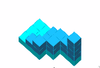
and then record them in a table like
we can then add to the first row, add to the second row, and to the third row to obtain strictly increasing columns to obtain the second diagram (in fact it is better to add to the first row and so on). Then if we consider , we obtain the formula
3.4 General Theory of Representations
Consider a compact connected Lie group . We will understand in terms of a maximal torus and the roots, which are the eigenvalues of the adjoint action of on . Here, is called the rank of . We know that compact connected abelian Lie groups are tori already, but we also need to show that maximal tori actually exist. In particular, we will see that any maximal torus is its own centralizer. First, observe that the closure of an abelian group is abelian. Next, we have a result due to Cartan.
Theorem 3.4.1 (Cartan).
Any closed subgroup of a Lie group is a Lie subgroup.
Proof.
Consider the exponential map . Then define by
This is a vector space because
and is closed. To see that is a Lie subalgebra, write
where and then note that because so is . Now we need to show that is (locally) the image of , where is the simply-connected Lie group with Lie algebra . We simply need to show it is a submanifold. Near , consider the quotient . Then if near , then there exist where such that . Now take a convergent sequence among the . We have
and then note that the integer part is in and the fractional part converges to . □
Proposition 3.4.2.
Maximal tori are in one-to-one correspondence with maximal abelian subalgebras.
We will give two different proofs of this fact.
First Proof.
Let be maximal commutative of dimension . Then we have a morphism of Lie groups, so we need to prove the image is closed. If the image is not closed, then its image is a closed connected abelian subgroup of dimension strictly larger than . Thus its Lie algebra strictly contains and is abelian, and this contradicts maximality of . □
Second Proof.
Let be a Lie group (or an affine algebraic group). Let be a subalgebra. Then let be the Lie algebra of the minimal closed subgroup such that . Then we will show that
To prove this, consider
This is a closed Lie/algebraic subgroup. Next, we see that
This implies that . Now we do the same for
This contains because and therefore and thus . □
Now consider the following observations:
- 1.
has no continuous automorphisms because is discrete. Then we have an exact sequence
is exact. We know that by maximality, and in fact we will see that . In addition, we know that is discrete and compact, and hence finite.
- 2.
Because has only countably many Lie subgroups, we have
Theorem 3.4.3.
Let be a maximal torus. Then
- 1.
Any element is conjugate to an element of .
- 2.
Any is conjugate to an element of .
Corollary 3.4.4.
All maximal tori are conjugate.
Proof.
Let be a different maximal torus. Then choose such that . Then by the theorem, there exists such that . Thus and thus and maximality implies that this is actually an equality. □
There is a general principle for proving theorems of this kind. If , then is the same as and thus as sets. This implies that has a fixed point on the manifold . More generally, a subgroup being conjugate to a subgroup of is equivalent to fixing a point of the manifold .
Now we consider the flag manifold (or flag variety) for . For , we see that is the centralizer of a generic diagonal matrix. We can describe as the generic class in either or . This is alternatively the moduli space of orthonormal frames in . Equivalently, this is the moduli space of flags (hence the name flag variety).
If I draw the flag red, will it be too communist? I don’t want to offend anyone. A. Okounkov
It is easy to see that acts transitively on the flag variety and that the stabilizer of a given flag is the group of upper-triangular matrices (known as the Borel). This implies that the flag variety is a compact complex manifold. For example, we see that . A key property is that the general flag variety has a cell decomposition into -many cells, each of even dimension, called Schubert cells. In particular, this means that . Next, if is homotopic to the identity, then a very special case of the Lefschetz fixed-point formula says that
where the multiplicity is the intersection number in . Because , there must exist a fixed point of positive multiplicity. Therefore, because any element of is homotopic to the identity, it must have fixed points on counting multiplicity.
We will prove that any element of a compact connected Lie group is conjugate to something in a maximal torus. Consider the adjoint action of a fixed maximal torus (or its Lie algebra ) on . Then the adjoint action of on splits into a direct sum of eigenspaces with nontrivial eigenvalues the roots. Thus we have
Now choose generic such that for any root . We want to prove
Theorem 3.4.5.
Any is conjugate to an element of .
This is implied by
Proposition 3.4.6.
Any is conjugate to an element that commutes with .
Proof.
Consider the adjoint orbit of , which is a compact smooth manifold. Consider a function on where, is the invariant metric on . Because is compact, has a critical point and thus vanishes on the tangent space to that point . This is the span of for . Thus there exists such that for all , we have
and thus . □
We remark that gives a -equivariant isomorphism . Even without this form, one can still talk about , which is a very important object. In fact, the Lie bracket on gives a Poisson bracket on .
Definition 3.4.7.
A manifold is a Poisson manifold if there exists a Poisson bracket is the structure of a Lie algebra on functions that is compatible with the product by the Leibniz rule. Here, this means that
If the product is commutative, this means that we have a derivation of the product and thus we have a vector field.
Note that has coordinates . Thus we can extend from by the Leibniz rule, and this turns into a Poisson manifold. This is known as the Lie-Kirillov-Kostant structure.
For a Poisson manifold , the span of satisfies the integrability criterion. The Jacobi identity tells us that that
Then the integral manifold passing through is called the symplectic leaf of and is a locally closed submanifold of .
On , we consider the subspace , and thus the integral manifold is actually the -orbit of . This orbit is called the coadjoint orbit and is equal to the adjoint orbit for compact groups.
Then we have for every symplectic leaf
and therefore is an isomorphism. Thus the map gives us a -form on which is antisymmetric by the axioms of the Poisson bracket. Now the axioms of the Poisson algebra mean that is closed, and thus the leaf is a symplectic manifold.
Definition 3.4.8.
A symplectic manifold is a manifold with a closed nondegenerate -form .
Theorem 3.4.9 (Kirillov-Kostant).
Coadjoint orbits of a Lie group are symplectic manifolds.
Now we will discuss connections to Morse theory. The idea is that a Morse function (function with all critical points nondegenerate) on a compact manifold tells us a lot about the topology of the manifold. Here, a Morse function is precisely a function where implies is nondegenerate. An example of a Morse function is the height function on a torus:
Now we can rebuild the manifold by gluing on handles, which are , where is the dimension of the manifold and the attaching map is on the part. This allows us to reconstruct the torus as follows:
Here at each critical point we are gluing a -handle, where is the index. From the symplectic point of view, the main property of is that the index of any critical point is even. This gives us a cell decomposition into cells of even dimension, and therefore .
Corollary 3.4.10.
The centralizer of of is connected.
Proof.
Note that is a locally trivial fibration. Therefore we have an exact sequence
and thus . □
Note that by Hurewicz and that is in bijection with critical points of index . Because of the cell decomposition into cells of even dimension, we have . This also means that has a unique maximum and minimum.
Note that if is generic, then is a maximal torus. This is because for generic , we have . Thus generic adjoint/coadjoint orbits of are of the form .
Returning to conjugacy in a Lie group, we can either use the Lefschetz formula to conclude that has a fixed point on or we can write .
3.5 Poisson Geometry of Lie Groups
We will say some more about Poisson manifolds. Recall that these are manifolds with a Lie algebra structure on that satisfies the Leibniz rule. As a subclass of these, we have symplectic manifolds , where is closed and nondegenerate. Then the two maps
are inverse to each other. Locally, all symplectic manifolds look the same, and there are always such that . This is a remarkable contrast to the Riemannian case, where Riemannian manifolds have local invariants such as curvature. On the other hand, Poisson manifolds may locally be very complicated. For example, if vanishes at , then the next term looks like a Lie algebra, so the classification of Poisson manifolds looks like the classification of Lie algebras. Thus we will focus on symplectic manifolds, which originated in classical mechanics. Here, the are coordinates and are momenta. Then the equations of motion in Hamiltonian form are
where the Hamiltonian is the total energy of the system. For example, if we consider a harmonic oscillator , then we have and thus
Therefore the orbits (going around a circle clockwise) of this motion are periodic with period . Now if we multiply by a constant, this will modify the angular velocity. Now if
then the motion will rotate each -plane with angular velocity .
In our case, our maximal torus acts on the (co)adjoint orbit . Now each -parameter subgroup acts via the Hamiltonian . Then the fixed points of this action are critical points of the function. We know is a fixed point if , where is also generic. Also, we may asssume that and . Thus fixed points of are the same as critical points of , which correspond to the Weyl group.
To compute the index of a critical point, we have , and so after complexification, we have
Because the roots come in complex conjugate pairs, we will have -dimensional representations that rotates with angular velocity . Now the Poisson bracket is
where is the -invariant inner product. By invariance, we know that unless .
Lemma 3.5.1.
If are roots, then .
Proof.
We have
More generally, if is a -module, then by the same argument. □
Further, the form is nondegenerate, so its extension to is nondegenerate. Also, by -invariance, we have unless , so with respect to this metric. Moreover, we have
where corresponds to the linear form via . To prove this, note that
Next, we have . Thus the sign of the Poisson bracket has to do with positivity of .
Because we have , then the Hamiltonian for the action of is
the index is even and is equal to assuming that . For any , we can define if . Then for any fixed point for some , this index is
And is equal to the number of hyperplanes separating from , which is the number of hyperplanes separating the positive cone from . This is also the length , which is the usual number of inversions (adjacent transpositions) for . In summary, the index of a critical point is always even and we have the following dictionary:
| Geometry | Algebra |
|---|---|
| Critical points | Weyl group |
| index | length |
Now we have a general statement: If acts by a Hamiltonian action on any symplectic manifold , then the index of any component of the critical locus is even. Geometrically, in the context of Morse theory, something like the below cannot happen:
In particular, every level set of is connected and is obtained by always attaching even-dimensional handles (and these have connected boundaries). Now if we have , the level set of is preserved by , so is connected when nonempty. By an argument of Atiyah, the image is a convex polytope, which is the convex hull of the images of the fixed points.
For instance, if is the maximal torus in and is the (co)adjoint orbit, then this pixks out the diagonal elements of a matrix in . For , the image looks like below:
3.6 Root Systems
Let be a compact Lie group and be a maximal torus. Then we know that
We will prove that the form a reduced root system and that . We know that the roots sit inside the root lattice, which sits inside the character lattice of , which is .
Definition 3.6.1.
A finite collection of vectors in Euclidean space forms a root system if
- 1.
For all roots , the vector
is also a root. Here is the metric on .
- 2.
For all roots , the quantity is an integer.
A root system is called reduced if for roots , the equation implies .
Note that there is an unreduced root system , where the form an orthonormal basis of Euclidean space. However, this does not appear in the context of Lie theory.
We will now classify root systems of rank . The only such root systems are and . The root system is the root system of with . Here, we have
To classify root systems of rank , we note that
This implies that is an integer. The simplest is called , with the two roots perpendicular. Next, the angle could be , and the root system is now , which is drawn below.
This is the root system of . The next root system, in the case where the angle is is the root system and , and it looks like
is the root system of and is the root system of . Next, we have the root system , which is drawn below:
In general, all finite, or even discrete, groups generated by reflections of can be explicitly classified. This restricts to the classification of crystallographic groups (which preserve a lattice), and inside this we can classify reduced root systems. This turns out to be the same as classifying compact Lie groups and complex reductive Lie groups.
The first step is for every , find . Last time, we showed that . Then we know . Now we can normalize this by . In fact, we will see that the form the dual root system in . Next, for any , we can choose , which defines an action of on . In particular, we have
Therefore a root corresponds to the submodule , and in particular, we have the submodule
and so is the unique vector of zero weight. Now we know the representation theory of , where the highest weights are integers. Also note that we only have even weights and a unique vector of weight , and thus the representation above is irreducible. However, by construction, it contains as a subrepresentation, so we must have
This proves that and that the are reduced. Also, we know that in the diagram
the representation is irreducible. These are reversed by , and thus acts by reflection on and . This implies that
Our next goal is to show that is generated by the . Before we do this, we will discuss the group generated by reflections. For example, if we consider an equilateral triangle, we can find a discrete group generated by reflections.
We can consider the connected components of the complement, and these are called polytopes. These can be studied in , and other spaces. Each of these is a finite intersection of half-spaces and is called a polyhedron. Then if are the reflections in the facets of , they generate a group . Now we can rephrase any word in the generators as a path, so for example, we have
Similarly, we can obtain by the procedure
Therefore, the group acts transitively on the set of chambers. In particular, any reflection is one of these reflections. Now there are some obvious relations on the :
- 1.
Clearly .
- 2.
If two hyperplanes have angle between them, then we have .
Theorem 3.6.2.
- 1.
This is the complete list of relations among the
- 2.
is a fundamental domain for .
The idea of the proof is to remove intersections of hyperplanes of codimension at least . This is still simply connected, but it has a map
which is a covering, and therefore it must be an isomorphism.
To say some more about , if is generated by relations, recall that corresponds to critical points on with index . Then we will see that for a vector , the relation if and only if gives us a chamber for . Therefore by the action of we can change the index to be , but there is only one cell of index because is connected.
Recall that if is a discrete group generated by reflections, a chamber is a connected component of the complement of the reflecting hyperplanes.
Theorem 3.6.3.
- 1.
For a chamber , is a fundamental domain for .
- 2.
is in bijection with the set of chambers.
- 3.
is generated by the reflections in the walls of with the relations and whenever the walls have angle .
Last time, we proved that the generate , Next, by the following picture, we see that words in generators correspond to paths in the set of chambers:
Proof.
We will view words in the generators of a group as the Cayley graph. This is the graph with vertices the group elements and edges if . Because , we don’t need these orientations. Now let
be given by . This takes the Cayley graph of to the adjacency graph of chambers. We will prove this map is an isomorphism. This will imply that and that acts freely on the set of chambers. In fact, we will beef it up to a covering map of something simply-connected.
Consider the complement of the codimension strata in . Also consider the set
where we identify with . This is clearly a local isomorphism near points on codimension strata, and therefore is an isomorphism because the target is simply connected. □
Example 3.6.4.
Consider the triangle groups . This is the reflection group of either generated by a triangle with angles . Here, the cases are
For example, consider the triangle generated by three perpendicular great circles on the sphere. Each angle is . In , we can consider the tiling of the plane by usual equilateral triangles, and in the hyperbolic plane, the fundamental domain of the action gives us a triangle.
In these cases, we know is
- •
Finite if .
- •
Infinite of growth like for .
- •
Infinite of exponential growth if .
Recall that the Weyl group is a finite group.
Theorem 3.6.5.
is generated by the for all roots .
Proof.
Identify with the critical points of on the orbit of in for a generic . We need to prove that there exists no such that is in the same chamber as . On the critical point , we will compute the index of the function . We know this is the number of roots such that and , which is the same as the number of hyperplanes separating and . This also equals the number of reflecting hyperplanes separating from , which is the length of .
Therefore, if there exists in the same chamber as , then there is more than one maximum of . However, because there are no -cells, the orbit of is disconnected, which is impossible because is connected. □
Now we have the following correspondence:
Discrete reflection groups in can be classified, so from this we can infer a classification of root systems. Next, the map from compact groups to root systems is an isomorphism, so compact groups (or complex reductive groups) can be classified. The conclusion is
- •
There are four infinite series denoted by corresponding to the different Dynkin diagrams.
- •
There are several simple exceptional groups: . As a representation of , we have . Note that has an outer automorphism, which is . From this decomposition and the root system, one can reconstruct the remaining brackets.
Now a Dynkin diagram is a diagram with vertices the and an edge between and when and no edge when . When , we have to choose which edge is longer, so the Dynkin diagrams are
4 Bonus: and algebraic surfaces
Recall that algebraic curves (or compact Riemann surfaces) come in three forms: (genus , Fano), elliptic curves (, Calabi-Yau), and curves of genus (general type). Each of these exhibits very different behavior when we consider meromorphic differentials . Then if we consider the canonical class . For any two meromorphic differentials , we see that is a rational function, so all forms define the same element of . Also, we can compute using Riemann-Roch that .
For example, on , the form has a double pole at infinity. Then if we consider a rational function , we can consider the form and then compute the degree using Riemann-Hurwitz. This implies that when , has negative degree, when , the degree is zero, and when , the degree is positive.
For general algebraic varieties , we can consider the canonical divisor associated to a meromorphic top form. Now let be a smooth projective surface in .
Example 4.0.1.
The simplest such is , and we can consider the form on , and this will have a triple pole at the line at infinity. Alternatively, if we consider the form , this has poles on the toric boundary. This implies that , which is the hyperplane class.
Example 4.0.2.
Let be a surface cut out by a polynomial of degree . When , we have a quadric surface, which look like this:
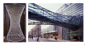
This has two families of lines parameterized by , and in fact, . Note that this is birational to but is not isomorphic. Projection from a point is a map and is an isomorphism outside of the projection point and the two lines through it. In fact, to resolve the base point of this map, we need to blow up . The two rulings through are contracted. Here, blowup replaces a point by a line representing all tangent directions through it.
In the toric picture, blowup and blow down are represented by the following:
Then we obtain because the hyperplane section is the sum of two .
In general, we can compute the canonical class of a hypersurface using the adjunction formula. We can write and thus we have
For example, if , we see that . This tells us that
- •
When , the surface is a del Pezzo surface.
- •
When , we have a K3 surface.
- •
When , we have a surface of general type.
When , the surface is a cubic surface and looks like this:
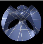
Over , every smooth cubic surface has lines. We have and thus , which is ample. Recall that a divisor is ample if some multiple of it defines an embedding into . Now there is a map from the Picard group to the Neron-Severi group, which is the group of divisors modulo numerical equivalence. Here, we need the intersection form , which is additive, invariant under deformation, and counts intersection points with multiplicity when is discrete and are effective. Here are some basic results:
- 1.
The Neron-Severi group of a surface is a free abelian group , and is called the Picard rank.
- 2.
The signature of the intersection form is .
Inside the cone where , we can consider the ample cone of ample divisors. The dual of this is the closure of the effective cone. There are effective divisors with negative self-intersection, for example any line on a cubic surface.
Now we may prove that the cubic surface is rational. To do this, we choose two skew lines . Now for any points , we consider the line through in , and there is a third intersection point. This defines a birational map , and in fact is the blowup of at six points. When we blow up, we obtain , and thus we have . Thus is very ample and defined an embedding into .This tells us that
If is in the closure of the ample cone and is a curve, we will consider how small can be. By the adjunction formula, we have
Therefore, we have . Thus we have and this is positive when is ample. This implies that , and this happens when . If , then is a line and can be contracted by Castelnuovo’s criterion, and when , we can contract this to an singularity (or ). If we consider the perpendicular of , then all -curves are:
- •
;
- •
;
- •
.
This gives us the lines on a cubic surface: the six exceptionals, the strict transforms of the lines between two of the blown up points, and the conics passing through five of the six points. The -curves are:
- •
;
- •
;
- •
;
- •
.
The first corresponds to blowing up a point twice, the second corresponds to blowing up three points on a line, and the third corresponds to blowing up six points on a conic. The last one corresponds to a cubic with a double point at and seven more points. The last ones correspond to the roots of . To see this, if we consider a singular and nearby nonsingular , we have a vanishing cycle in , which is a root. If we consider the monodromy, this is exactly the reflection in this root.
This defines a map from to the family of all nonsingular cubic surfaces. Unfortunately, we did not get to the punchline, which was to actually choose a set of roots in this cohomology.