Integrability, enumerative geometry, quantization
Integrability, Enumerative Geometry, and Quantization
August-September 2022
Notes by Patrick Lei
Lectures by Various
Simons Center for Geometry and Physics
Disclaimer
These notes were taken during the program using the vimtex package of the editor neovim. Any errors are mine and not the speakers’. In addition, my notes are picture-free (but will include commutative diagrams) and are a mix of my mathematical style and that of the lecturers. Also, notation may differe between lecturers. If you find any errors, please contact me at plei@math.columbia.edu.
Acknowledgements
I would like to thank Gaëtan Borot, Alexandr Buryak, Melissa Liu, Nikita Nekrasov, Paul Norbury, and Paolo Rossi for organizing this program.
Program Website: https://scgp.stonybrook.edu/archives/33309
1 Virasoro constraints in enumerative geometry (Alexei Oblomkov)
Here is an equation of a plane curve over formal power series in , which we will call the Lambert curve:
This curve appears in the work of Oblomkov-Okounkov-Pandharipande [OOP20] which treats the descendent Gromov-Witten/Pandharipande-Thomas correspondence in the stationary, non-fully equivariant case. The main question is to consider deformations of this curve.
We will now state the main formula of interest:
| (1.1) |
This formula lives on the curve , where for a compact threefold. Here, we define
The satisfy the usual Heisenberg relations .
Theorem 1.0.1 ([OOP20, Theorems 4, 5]).
There is an equality (after the standard change of variables and up to a monomial in ) of equivariant -legged vertices with descendents
modulo , where
where is the universal stable pair on the PT moduli space. Here, we have
1.1 GW/Hurwitz correspondence for curves
1.1.1 Hurwitz theory
Hurwitz theory counts ramified covers of a curve with specified ramification data:
Hurwitz proved that these numbers are always finite and that
where is actually in the center of . Then acts on by the constant function .
Because of this, we can write
This can now be computed by a hook length formula, which corresponds to localization in the Hilbert scheme of points on . If we fix , then the function
is a symmetric function on , or a so-called shifted symmetric function. If we consider the limit
this is a free algebra on functions satisfying . We now consider the functions
By the work of Vershik-Kerov, the shifted Schur functions can be written as
which after inversion becomes
We can also write the completed conjugacy classes .
Example 1.1.1.
For example, we have .
1.1.2 GW/Hurwitz correspondence
Theorem 1.1.2 ([OP06a]).
There is a correspondence
between Gromov-Witten descendents and Hurwitz objects, where is the class of a point. More precisely, we have
This can be related to PT theory as follows: consider with the antidiagonal action of on and recall that . Then we have the localization formula
The left hand side becomes
where .
1.1.3 Pandharipande-Thomas theory
For a threefold , Pandharipande-Thomas theory [PT09] considers moduli spaces
of stable pairs, where is a pure dimension sheaf on supported on and . This has technical advantages over the older Donaldson-Thomas theory, one of them being that we don’t have to study the Hilbert scheme of points on . If we let be the universal stable pair, then we define
for any .
Now consider . Then the first nonempty PT moduli space is
If we let , we define
where is the universal ideal sheaf on .
1.1.4 Idea of proof of GW/Hurwitz
We begin with a correspondence between relative Gromov-Witten theory without descendents and Hurwitz theory. Then we can degenerate our target curve with descendents to bubble out the descendents. We now need to show that
which requires us to study the equivariant Gromov-Witten theory of .
1.1.5 Fock space
We begin by defining the infinite-dimensional space
Then the semi-infinite exterior power has basis , where such that
- (i)
The set is finite;
- (ii)
The set is also finite.
Then we write .
If we rotate the French way of drawing Young diagrams counterclockwise by , we obtain the Russian way of drawing Young diagrams:
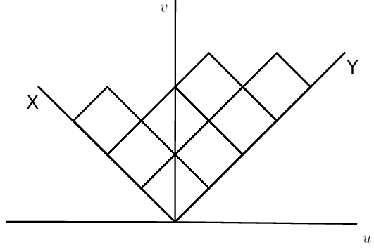
There are two natural statistics associated to Young diagrams as in Figure 1.1, which are the size and where the vertex touches the bottom. Define
We now define the operators
Then we have
We can check that and . If we consider , then assigning gives a projective representation of . The Casimir operator is , and this acts by
In addition, the operator acts by
Define the operators
where . In particular, we have for , where .
The space has two natural bases given by the and by . The transition function between them is . This appears in the Gromov-Witten theory of :
where the last equality uses the formula . The last formula we will write in this section is the relation
1.2 Equivariant Gromov-Witten theory of
We are interested in an equivariant version of the GW/Hurwitz correspondence, so we want to compute the Gromov-Witten invariants
where the are Getzler descendents, is the operator in Theorem 2.1.1, and is ramification data over .
1.2.1 Localization in Gromov-Witten theory
Focusing on the case of , we will discuss localization. We begin with the moduli space of disconnected stable maps, and the fixed points
with respect to the action are simply a moduli space of bipartite graphs with extra markings on the vertices (genuses and marked points) and the edges (degrees ) subject to various conditions, for example
Then recall that and .
In particular, we see that
so we need to consider integrals over this space.
One standard technique is to cut the edges in half and consider the vertices and then glue the edges together, and this puts the markings and the degree copies of on the same footing. We now need to compute the contribution of a vertex to our integral. We want to compute the contribution of to
which is in fact
1.2.2 Hodge integrals
The main component of this computation is the terms, which are called Hodge integrals. Let
be the universal curve on the moduli space of curves. Then
is a rank vector bundle, called the Hodge bundle. Then let be the Hodge classes and be the psi classes. The Hodge integral is now
There is a connection between Hodge integrals and Hurwitz numbers in the nonequivariant case, due to Ekedahl-Lando-Schapiro-Vainshtein [ELSV99]. The main contribution of Okounkov-Pandharipande [OP06b] is to replace the Hurwitz numbers in the equivariant case. First, we consider , which counts genus curves with simple ramification at and ramification data at , where
by the Riemann-Hurwitz formula. By ELSV, this number is computed by the formula
Our next goal is to interpret in the Fock space analytically. Write
where
is the Pochammer symbol. In the case where and , we obtain
Keeping as the number of simple branch points, we obtain
Lemma 1.2.1 ([OP06b]).
We have the identity
where we use the formula
We will also discuss some more properties of the . First, there is the identity
and second
Example 1.2.2.
We have an explicit example of a Hodge integral
with two insertions.
1.2.3 Application to Gromov-Witten theory
Returning to the vertex contributions, we obtain
If we let be the projection operator on and write it explicitly as
then we obtain the formula
When , the formula simplifies to
1.2.4 Dressing operator
Recall that we want to compute the Gromov-Witten invariants with Getzler descendents, which are given by
It remains to describe this matrix and the variant . Here, the are defined by
so for example we have
We will work in . We also write
where and , so . Then define the operator
Both the operators live in . Then we will have .
Lemma 1.2.3.
Write , , and . Then there exists a unique solution to the equation
such that
- 1.
;
- 2.
;
- 3.
is upper triangular.
Sketch of proof.
We will compute the derivative
and this implies that . Some more “basic checking” completes the proof. □
Remark 1.2.4.
The operator in the lemma was discovered by a computer and it is unclear why it appears.
Theorem 1.2.5 ([OOP20]).
We have the formula
Proof.
Define the operator
and define analogously. In fact, we have and
Thus we obtain . Differenting both sides by , we obtain the desired result. □
1.3 GW/PT correspondence
Let be a threefold and consider Pandharipande-Thomas theory on , which we defined in Section 1.1.3.
Example 1.3.1.
Example 1.3.2.
Consider . We will consider the moduli space . If we consider the torus preserving the symplectic form on , then the virtual class satisfies
1.3.1 Descendents in PT theory
Let be the universal stable pair on . Then if , we define
When , then
Then there is the formula
Of course, if acts on with the antidiagonal action, we see that
where . Then we have , and so
The term comes from the presence of the Todd class. Recall the definition
where .
Now the main formula is that for , we have
On the Gromov-Witten side, we have
This allows us to solve the GW/PT correspondence and match descendents, where
This actually allows us to define negative descendents, but to match the descendents we need to write in terms of the .
1.3.2 Matching GW and PT descendents
Our method will be to do the following:
- 1.
Diagonalize ;
- 2.
If is diagonal with eigenvalues
then acts on by
There is a boson/fermion correspondence between
The first step is of course to diagonalize (for simplicity, we will set ). Clearly we can identify
Then we know
so we need to solve the differential equation . The solution is
To make this work, we need , and to diagonalize we take the basis
where . The Lambert curve is obtained from , which produces the curve
Remark 1.3.3.
Recall the dressing operator , which we defined using a differential equation. An explicit formula for is
An upgraded version of the GW/PT correspondence is the following:
Theorem 1.3.4 ([OOP20]).
Subject to , there is an explicit equality of descendent vertices
Remark 1.3.5.
Using the Pandharipande-Pixton philosophy, we can obtain equality Theorem 1.0.1. This will be enough to prove the stationary GW/PT correspondence for toric varieties.
1.3.3 GW/PT correspondence with descendents
Recall that on the Gromov-Witten side, the insertions of interest are , while in PT theory, the corresponding insertions should be . This correspondence was proved in [MOOP11] for any toric variety and any , while Pandharipande-Pixton [PP17] prove this for a complete intersection in . There is also a conjectural equality between and .
More generally, [MNOP06b] conjecture that there is a series of “chemical reactions” that take to an expression involving with Chern classes.
Pandharipande-Pixton [PP14] consider the operators
in the fully equivariant case. This fits into an overall picture
Theorem 1.3.6 ([PP14]).
- •
The operator is rational in ;
- •
The operators and are upper-triangular.
- •
There is an equality
for any and any .
While is unknown, there is an explicit formula for some of the matrix elements, which we call .
Theorem 1.3.7 ([OOP20]).
There is an explicit equality
for any toric and stationary descendents .
We will consider the formal algebras
Then write
Then we can write
The are quite complicated, but in a simple case, we have
There is a bumping and splitting that produces things like
where . We will take the and to have degrees , respectively.
1.3.4 Virasoro constraints in PT theory
For a toric variety , we can apply the GW/PT correspondence to the Virasoro constraints for . This obtains Virasoro constraints for , which turns out to be quite simple. The Virasoro constraints in PT theory are:
- •
We have
for any . For example, .
- •
The constant terms are
- •
There are also the operators satisfying
and operators .
Theorem 1.3.8 ([MOOP20]).
For any , we have
Conjecture 1.3.9.
The theorem holds for all descendents .
The proof essentially amounts to checking the following formula:
Theorem 1.3.10.
There is the formula
Here, is the usual Virasoro for Gromov-Witten theory.1 The only contribution to descendents of to are
Therefore, we can define and .
Proposition 1.3.11.
- •
The operator preserve stationary descendents, as in
- •
We have the vanishing
for all .
Let be a surface and . Then
and so the virtual class is
Then if is the universal ideal on the Hilbert scheme, define
Corollary 1.3.12.
For any toric surface and , we have
Proof.
This follows from
□
Remark 1.3.13.
A cobordism argument was used by Moreira [Mor22] to extend this to any surface with .
2 Counting curves in 1, 3, and 5 dimensions (Andrei Okounkov)
The main object in Gromov-Witten theory is the moduli space of stable maps from a curve to . This is of course highly disconnected, so the genus component will be weighted by while we will hide the degree component for now. One of the major ideas in this subject is to push forward cohomology classes to the moduli of curves, which forms a cohomological field theory with rich structure coming from maps between different moduli spaces of curves. Instead, we will push things forward to . Just like we can vary the source curves in families, we can degenerate . Also, automorphisms of still act on our moduli space.
Our goal is to give a target space description of integrals over . We would like a geometric theory that reproduces the same integrals and an algebraic theory that computes them in some fashion resembling a topological quantum field theory – for example Chern-Simons theory.
The most basic degeneration of a variety is to degenerate
where is a smooth divisor shared between and as in Figure 2.1. If we write , we obtain the relation
in algebraic cobordism. As proved by Levine-Pandharipande [LP09], this relation generates all relations in algebraic cobordism. A similar type of degeneration is the expanded degeneration of Jun Li [Li01], which creates an accordion of -bundles as in Figure 2.2.
This fits well into the usual TQFT formalism where the boundary divisor is associated to a vector space and the manifold is a vector in this space. Because is usually the cohomology of some nice space, it has a product , integration, and a form
We can impose conditions at by either pulling back cohomology classes from or pushing forward to a cohomology class in .
In reality, we have more general degenerations, where we have a degeneration
where the are glued along a simple normal crossings divisor. This has been extensively studied in geometry, for example in logarithmic Gromov-Witten theory, logarithmic Donaldson-Thomas theory of Maulik-Ranganathan [MR20], and Brett Parker’s “exploded manifolds” [Par12].
2.1 Counting curves in 1 dimension
Now, we will take , so we are studying maps from a curve. We can take or even with the action of . Before we begin, we would like to discuss why we prefer to be odd. If we consider , then
where is a coordinate on . This can be removed by taking , but doing so is very hard and introduces new problems. However, Mumford tells us
and thus changing dimension by is very easy.
In the case of , the geometric target space theory is just Hurwitz theory, which as in Section 1.1.1 counts ramified covers of of degree with specified ramification data. This ramification data is an instance of a relative condition in Gromov-Witten theory, which is as follows. We can consider the moduli space of relative stable maps , where we impose that , where is a partition and the are the marked points of .
Hurwitz theory has moduli spaces parameterizing maps which are ramified covers with the specified ramification, where can vary in moduli. These moduli spaces are finite over the moduli of curves, so the most interesting number is simply the degree of this map, which is the Hurwitz number. Under degenerations , then the ramification at the node should match. These are called admissible covers; see Harris-Morrison [HM98] for a reference. This gives us the relation
where . This insertion is inverse to the the pairing on .
The general answer for Hurwitz numbers was known to Frobenius and Burnside as
This contains a blueprint for the modern understanding of all 2d TQFTs as well as handle-gluing operators.
2.1.1 More algebraic way to think about characters of
There is the action of a central extension of on , known as the Fock space. We need the operators defined in Section 1.1.5, but we also want the Heisenberg operators
which act on the vacuum by
We also want co consider the fermionic operators
taken without the normal ordering and -regularized as in
The operator acts with eigenvalue
on . By Vershik-Kerov and Kerov-Olshanski, the central character of and are polynomials of , which are and in fact is equal to
where the lower order terms are controlled by the Gromov-Witten/Hurwitz correspondence. In particular, there is the remarkable formula
while the case of the elliptic curve is simply the trace of the middle operator without the terms.
2.1.2 Gromov-Witten/Hurwitz correspondence
There are several features of this correspondence:
- 1.
There are no descendents of or in Hurwitz theory. In Gromov-Witten theory, these can be explicitly reduced to descendents of .
- 2.
Relative conditions correspond to relative conditions. This will always be true in the things that we study.
- 3.
Descendents of are equal to relative conditions glued on a bubble.
This reduces to computing everything in the Gromov-Witten theory of , where one of the marked points is descendent and the other is relative.
The remarkable formula in Theorem 1.1.2 can be computed explicitly and gives a formula for the completed cycles as conjugacy classes. More generally, if we have two relative points, the invariants can be computed explicitly and are B/C-symmetric in . In particular, for , we have
and this was computed by Faber and Pandharipande [FP00].
We now want to consider the equivariant theory for .
Theorem 2.1.1 ([OP06b]).
We have the identity
where we take a linear change of times determined by
2.1.3 Role of integrable systems
This last formula was found by Getzler [Get04] and is problematic in the limit. Morally, the Gromov-Witten descendents give a quantum integrable system that looks like a free boson or free fermion. By the Kyoto school of integrable systems, there is a classical integrable system for generating functions. In particular, for with two marked points, the degeneration gives us
which is a tau function for the 2-Toda hierarchy and in particular gives a KP hierarchy for linear Hodge integrals in degree .
Remark 2.1.2.
These equations differ from the equations found in 2009 by Kazarian [Kaz09], and this is not well-understood.
Fundamentally, these equations come from Plücker relations for . This is because in there is an invariant operator commuting with . Our goal now is to understand the deformation of the following for :
- 1.
The group ;
- 2.
The representation ;
- 3.
The quantum integrable system;
- 4.
The invariant operator in .
2.2 Counting curves in 3 dimensions
Again, we are looking for a target space description of enumerative theories, but this time for threefolds. Here, we will consider Donaldson-Thomas (sheaf-counting) theories on a threefold . The connection to Gromov-Witten theory was conjectured by Maulik-Nekrasov-Okounkov-Pandharipande [MNOP06a; MNOP06b] building on the work of Aganagic-Klemm-Marino-Vafa [AKMV05] and the connection to box counting by Okounkov-Reshetikhin-Vafa [ORV06].
2.2.1 Donaldson-Thomas theory
While Gromov-Witten theory thinks of a curve inside as a map , Donaldson-Thomas theory thinks of as being cut out by the ideal sheaf
which has discrete invariants the degree and the holomorphic Euler characteristic . This has a natural obstruction theory
which is unsuitable for our purposes. Instead, we interpret as a rank torsion-free sheaf with
and so we obtain the obstruction theory
There are no higher Ext groups (even for orbifolds) by a result of Zhou [Zho18].
In Donaldson-Thomas theory, the descendents are , where is the universal sheaf on . We would hope that counts in fixed degree (this does work) and fixed genus (this does not work because moduli spaces are empty for or ) may be related, but unfortinately this is too naive. Instead, we expect a GW/DT correspondence
after the standard change of variables
where is weighted by and is weighted by genus.
All moduli spaces in Donaldson-Thomas theory are schemes, so all DT invariants are actually integers. If we want actual equality of analytic functions with the Gromov-Witten partition function, we must have rationality of the DT partition function (this is related to BPS integrality). For this all to work out, the virtual dimensions
must be the same, so must be a threefold. Of course, our correspondence requires
- 1.
Identification of descendents;
- 2.
Division by degree contributions in DT theory;
- 3.
Prefactors like .
See [Oko19] for precise formulas and additional discussion.
In DT theory, it is possible to remove the degree terms geometrically using Pandharipande-Thomas theory, which was discussed in Section 1.1.3. Some parts of identifying the descendents are easy (for example primary descendents and relative conditions are fine).
2.2.2 Relative conditions in DT theory
In Gromov-Witten theory, a relative condition for a divisor consists of specifying a condition like
If and are mapped to the same point with tangent to , then we have an evaluation map to the inertia stack of , where we remember the ramification data on . Therefore, we are really integrating orbifold cohomology classes, where classes in are colored by integers, so we are considering
If we want to resolve the tangency, then we must degenerate in a family and bubble off of -bundle on (or a whole accordion).
In Donaldson-Thomas theory, we have a map
which is regular as long as multiplying by the equation of is injective. To ensure this, we must bubble out the accordion as above. Therefore, the relative conditions come from , which has a Nakajima basis
where the vacuum vector is . Of course, there is an isomorphism
and so adding a subscheme of length along should correspond to tangency of order along .
The GW/DT correspondence has been proved for many, but not all, threefolds, and a key step, as in Maulik-Oblomkov-Okounkov-Pandharipande [MOOP11], is to consider a fibration
where is a crepant resolution of , where acts with weights . Thus is a crepant resolution of
When , then is a local curve, so for example is fine, and we should recover Hurwitz theory for .
Remark 2.2.1.
ADE surfaces are special for many reasons, for example enhanced symmetries of or of .
The torus fixed points on are those curves supported on , which can be thought of having a partition on (corresponding to the closure of the generic point) with some extra boxes. The DT analog of the Mumford relations is that if , then the virtual class vanishes for all nonminimal cases. Of course, the fixed points of correspond to partitions. If , then
where are the arm and leg lengths respectively. Then we obtain
and so the virtual class is
When , this becomes
This clearly is related to the representation theory of the symmetric group.
Remark 2.2.2.
Subsequent to [MOOP11], a different perspective was developed, in particular for computations in K-theory. Unfortunately, we cannot say anything about a possible relation to Gromov-Witten theory.
2.2.3 Role of quantum groups
If we return to our -bundle over , we want some kind of cohomological field theory on the stack of -bundles on curves (which can vary in moduli). This has various building blocks related to with a descendent at and relative condition at with the action. The descendent conditions correspond to
while the relative conditions correspond to
By the ideas of Nekrasov-Shatashvili [NS09], this structure should be described by a quantum group, and this idea has been realized (also in K-theory) with the quantum group in K-theory and the Yangian for cohomology. Here, if are the weights of acting on , then is the weight of the symplectic form. There is a noticeable difference between and , and it becomes more dramatic for other quivers.
Remark 2.2.3.
In order to work with these objects, it is important to use a computer, and we would like to advertise the code written by Henry Liu: https://github.com/liu-henry-hl/boxcounting.
Remark 2.2.4.
If we restrict to , then
as a Hopf algebra, so we recover our description of Hurwitz theory.
Example 2.2.5.
Recall that the operators corresponding to with one descendent and two relative conditions commute. These should be Baxter -operators, and this is more or less true.
2.2.4 Quantum loop algebra
The quantum loop algebra is a Hopf algebra deformation of . The original loop algebra has a loop rotation automorphism, where if is a representation, is the precomposition with . The way we will construct our quantum group is by using the category of modules, which for a Hopf algebra have tensor products and duals. There are particularly important maps. where for , we take
and for we take
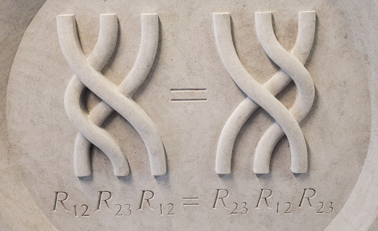
This is a rational operator, and it must depend only on if the loop rotation is an automorphism. If we have three representations , then there are two ways to reverse the order, and the equality between them is called the Yang-Baxter equation, see Figure 2.3.
Finally, we would like to reconstruct our quantum group given a family of -matrices. We will do this using
We can always assume that the collection of are closed under the tensor product. If we consider a physical space and auxillary space , then matrix elements in give operators depending on in . These operators will generate and are closed under product (two auxillary spaces, one physical) and coproduct (one auxillary, two physical). Morphisms in the category of modules are maps commuting with -matrices, and so we obtain relations in . The -matrix indeed gives braiding and commutation relations by the Yang-Baxter equations.
Now we will consider a family of subalgebras, called Baxter subalgebras. Let be such that . These come from the Cartan torus, which in geometric cases come from discrete invariants. Then we consider the transfer matrix
These commute for fixed and all , and so we get a family of commutative subalgebras in which are parameterized by a maximal torus in .
More generally, we can have several strands on a cylinder and one strand going around as in Figure 2.4 with the same condition on as before. But then we have commutativity with , and so we get a canonical flat -difference connection on , which is the qKZ equation.
2.2.5 Some more curve counting
We now want to return to curve counting on fibrations
where for now we will specialize .
We will begin with Gromov-Witten theory. For example, when , then is the total space of two line bundles on , so above there are curves collapsed to a point and above the base there are copies of mapping with degrees . Therefore we have something like
The triple Hodge integral terms (Figure 2.5) also involve nonsingular boundary conditions of tangency to (resp. ). Recall that we can break a curve in half while adding relative boundary conditions, and if we have with a action, it can be broken in half with nonsingular boundary conditions into .
On the other side, in DT theory, a half edge corresponds to a 3D partition with extra boxes.
The correspondences also include Givental’s -function for , which is of course a Nakajima quiver variety.
Of course, whenever the target is a GIT quotient (for example in the case of a Nakajima variety), there is a notion of quasimaps [CKM14], which for are actually equal to Pandharipande-Thomas moduli spaces [Oko17]. For , these are not PT moduli spaces, but there is still a correspondence with PT-like theories [Liu21]. The combinatorics of the PT vertex terms looks like Figure 2.6.
The half-edge solves differential and difference equations (giving quantum groups) and are a much evolved relative of the hypergeometric function of the form
where the are the Kähler variables (solving a linear differential equation) and the product term contains the equivariant variables (solving a linear difference equation).
2.2.6 qKZ equation
Donaldson-Thomas and quasimap theories make sense in -theory, and so we obtain a -difference equation from quantun groups, for example the qKZ equation. which comes from Figure 2.4. Here, the strands are and we will call the blue strand . Recall that
and so we have
where lives in the Cartan torus (also the Kähler variables) and the loop rotation is , where .
Consider unrolling the cylinder into a hyperplane arrangement. Consider the simple example of hyperplanes with walls like and , see Figure 2.7. We can move in three directions, and in the first direction we obtain
In the second direction, we obtain
More generally, from each wall in our hyperplane arrangement , we obtain an operator . If we consider such that for all , then translation by is conjugation by of all . This produces commuting -difference operators, which are transition functions for a vector bundle of the form
For example, for , we obtain the following:
- 1.
First, of course the qKZ equation, which depends on in the Cartan torus of .
- 2.
Universally, there exists a -difference connection in that commutes with the qKZ operator. Operators in act on . This was studied first by Etingof-Varchenko [EV02] for finite-dimensional Lie algebras , where the are simply the roots of . They write elements
and these are called quantum dynamical Weyl groups. More generally, Okounkov-Smirnov [OS22] consider more complicated arrangements, for example for , where we need all roots of of , and so the hyperplane arrangement is . This is clearly preserved by translation by , so the root subalgebras are
The way to prove the above is to
- 1.
Find qKZ among the -difference equations in the equivariant variables;
- 2.
Use commutation with qKZ and other known results to conclude.
We know that is a module over a quantum group. Then
where lives inside the space of rank framed sheaves on . Here, a framed sheaf is a sheaf on such that
Clearly, there is an action of on framed sheaves, so the sum of two ideals is the fixed locus of the maximal torus. Normalizing one of the weights of the torus, the locus of two ideals is the fixed locus of matrices of the form
and so shifts in give the qKZ equation.
Remark 2.2.6.
The Hilbert scheme is the Nakajima quiver variety for the quiver with one vertex and one loop.
Then the qKZ equation is
and comes from a twist by in the framing. In the case of for , there are more fixed points of and there are “constant sections” whose degrees are encoded in the Kähler variables.
2.2.7 Stable envelopes
We would now like a map
such that if we insert the relative conditions in the -fibration, all contributions cancel except those of the constant curves. Once this stable envelope exists, we will have
Vanishing is easier in cohomology [MO19], but is more difficult in K-theory. The reason for this is that vanishing in -theory is usually proved using rigidity (properness, which implies the result is a polynomial in , and a degree bound, which implies the result has negative degree).
The stable envelope is supported on the full attracting locus inside (or repelling for ), which gives properness. For degree bounds, the Newton polygon
is contained a fixed polygon.
Remark 2.2.7.
Rigidity in K-theory should come from a rigidity argument in elliptic cohomology, where K-theory is thought of as coming from a nodal degeneration of an elliptic curve.
More abstractly, let be a torus acting on a variety . Then we choose a chamber in , where the walls are weights on . This is a choice of attracting and repelling directions and corresponds to such that . Now for all adjacent strata in our chamber structure, there should be an attaching map, and the attaching maps should commute. These can be constructed with some assumptions on , and now the -matrix is simply the composition of one attaching operator and the inverse of the other. By the original commutation relation, we obtain the Yang-Baxter equation.
Example 2.2.8.
If we consider the rank sheaves and write , then there is an action of . Therefore,
More generally, for Nakajima varieties we can consider .
2.2.8 From enumerative geometry to quantum integrable systems
A quantum integrable system is controlled by a commutative subalgebra of
One interesting problem is to find the eigenvectors and eigenvalues of this algebra. The Hilbert scheme of can be replaced by some Nakajima quiver variety
where the framing is fixed.
The quantum integrable system is actually the limit of some flat -difference connection. In this setting, the problem of finding eigenthings is the problem of finding an integral solution to the -difference connection.
In the classical setting, consider a hyperplane arrangement and take hyperplanes
where the is fixed and the vary, then we obtain integrals that look like
where the are rational and the are homology classes on the complement of the hyperplane arrangement. This is like an Euler integral, which has the form
Our integral solves a differential equation (the Gauss-Manin connection) as well as a difference equation.
We now need to consider a -analog. Here, the will live on the complement of translates of subtori inside a tori, and the exponentials become gamma functions. Thus we are now integrating
which is a -analog of a Mellin-Barnes integral. These are fundamental solutions to the -difference equation.
The -difference equation has the form
In the limit, our solutions become
where is the eigenvector with eigenvalue . The eigenvectors and eigenvalues correspond to critical points of the term, where the eigenvalues are and the eigenvectors are given by evaluating at the critical points of . The are called the off-shell Bethe eigenfunctions and also depend on some auxillary variables. Note that we need to substitute in solutions of the Bethe equations
Remark 2.2.9.
There is an important detail in which it is better to do the replacement
Geometrically, we will work with quasimaps to Nakajima quiver varieties. The fundamental solution will correspond to the with one nonsingular point and one relative point. On the other hand, the vertex (see [Oko17, Section 7.4]) is the Mellin-Barnes integral.
Example 2.2.10.
Consider on . This has weight above , along the , and above . Therefore,
if , and so the Euler class is
which is a ratio of two -gamma functions.
The ideas in this example work more generally, and now it remains to find the elliptic term. This will come from some consideration of elliptic cohomology. The moduli space
of quasimaps (or for a general Nakajima variety) has evaluation maps
This gives us a push-pull morphism
This gives us an elliptic function which goes into the missing argument of the bottom-left . Also, the ratios of gamma functions were known to Iritani in the classical setting.
Remark 2.2.11.
The consideration of elliptic cohomology does not affect the gamma function terms of the fundamental solution. The gamma function terms control the spectrum and can be observed already in the case of just one nonsingular point. This was observed already in [NS09].
2.2.9 Elliptic cohomology
Recall that
where . If we consider the action of , we can consider the equivariant cohomology
This comes from the observation that has ways to lift to an equivariant class (consider each of the toric divisors). If we consider
this is the union of hyperplanes , which are the cohomologies of the fixed points. Lifting to -theory, we have the same picture after replacing with and taking instead of .
Returning to the case of Nakajima varieties, the ring
is generated by the tautological bundle and its exterior powers. Then its spectrum
is again a union of planes with data coming from plane partitions (which are the fixed points).
Finally, it makes sense to replace by , where all of the exact same equations hold (subject to writing the group operation on as multiplication). The elliptic cohomology of is drawn in Figure 2.8.
Remark 2.2.12.
It is important to note that is a scheme and not an algebra, so it is covariant in both and .
Note that if is connected, then
is the moduli space of semistable degree -bundles on the dual elliptic curve . Also note that .
2.2.10 Computations in elliptic cohomology of
In order to compute things, we need Euler classes. Suppose is a fixed point of acting on , is a vector bundles, and acts with weights on . Then
Note that these theta functions are not functions but are sections of line bundles on elliptic curves. Recall that is a pullback
This gives us a map
and on there is the theta divisor , which is the locus of bundles with a section. Pulling back to , we obtain a line bundle , which is where lives.
Pushforwards in the elliptc theory involve Euler classes and thus twists by line bundles. If we use localization, we obtain the factors in Table 2.1.
| In | In | In |
|---|---|---|
Then the pushforward gives us a map and the inclusion of a fixed point in gives us a map .
Remark 2.2.13.
There is an inclusion
The Kähler variables live on the left hand side, and quantum computations in K-theory embed inside classsical computations in elliptic cohomology.
Remark 2.2.14.
In principle, one could study enumerative counts in elliptic cohomology or even in another complex oriented cohomology theory like complex cobordism (see [She16]). However, we cannot form generating functions in these situations (for example in elliptic cohomology everything lives on a different line bundle), so we want to study the difference equations directly without generating functions.
We want to actually compute with the line bundles for vector bundles on . For the tautological bundle, we have
For the tangent bundle, we obtain
Note that if we restrict , we have a square root. Thus, we can find a polarization
Thus we will need sections of a line bundle of the form
We will call the determinant . Recall that taking the determinant corresponds to taking
Now recall that , so for (the Kähler variable), we can consider the meromorphic section
of some degree line bundle. More generally, we can take .
Recall that we have a map
We want to take a Lagrangian class on and extend it to the ambient stack. This is like taking a section of a line bundle on and extending it to the ambient stack. The ambient stack has a Harder-Narasimhan stratification in which the stable locus is the first piece. This allows us to take an inductive approach to the interpolation, see [Oko21]. There is a nonabelian analogue of this, see [Oko20].
One step of the induction is the following. Consider the inclusion . Then in ordinary cohomology, we have the long exact sequence
By Atiyah-Bott, the normal bundle has a nontrivial action, so all of the connecting maps vanish. By excision, we can replace by an embedding of into a vector bundle over , which produces
In elliptic cohomology, we obtain an exact sequence of line bundles. Consider the diagram
This produces us an inclusion , which gives us the divisor on . From a section of , we have an exact sequence
In studying sheaves on , we want global sections. Consider the long exact cohomology sequence
Note that because , has degree . It is also nontrivial (sections have poles related to enumerative geometry). However, if is a nontrivial degree line bundle on an abelian variety , it has no cohomology whatsoever.
We have now produced a stable envelope
which interpolates sections of line bundles. We also have the traditional elliptic stable envelope [AO21]
As we change attracting and repelling directions, we obtain elliptic -matrices. The K-theoretic and cohomological versions can be obtained using degeneration.
2.2.11 Quantum q-difference equations
We would like to solve these equations using integrals. Recall that in K-theory, we have
Recall that the solutions are of the form
As , the gamma functions give the Bethe equation, while the are the limit of the in [AO17]. This is called the off-shell Bethe eigenfunction. For quotients by groups of the form , the nonabelian stable envelope reduces to the abelian one, so there is a formula in terms of -matrices.
Consider the spin chain, where we have states like . Take the vacuum to be . Then the physical diagram will look like Figure 2.9.
If the spectral variables solve the Bethe equation, then the bottom state is an eigenvector. This is the origin of the algebraic Bethe ansatz.
In our setting, consider the picture of Figure 2.10.
The analog of all up arrows here is when and the maps are isomorphisms while the maps are zero. This happens because the Bethe roots sit inside a maximal torus of here.
2.2.12 An open problem
In dimension , we computed the equivariant in terms of the action of on the Fock space and concluded that the with two marked points is a -function for the 2-Toda hierarchy. This comes from the action of on , which has the action of
In dimension , we know both the equivariant with one marked and one nonsingular point and with one marked point and one relative point in terms of . In the limit, we recover , which corresponds to going down to dimension. If we take acting on along with a screening operator, where
what is the deformation of 2-Toda?
The case of one marked point and one relative point is rational in [Smi16]. Three key facts are
- 1.
The equivariant with one descendent and one relative condition vanishes for for (the so-called large framing vanishing) [Oko17].
- 2.
Splitting the equivariant in half and adding two nonsingular points, consider , where is fixed and is large. Then acts on by scaling. We now have
so the descendent is a Laurent polynomial in the Chern roots of the tautological bundle . Twisting by , we obtain an ordinary polynomial. Localizing on and and taking , we reduce to computing the same descendent for .
- 3.
In the limit, the fundamental solution for the -difference equation becomes the product of an explicit fusion operator and two fundamental solutions.
3 Double ramification cycles and integrable hierarches (Paolo Rossi and Alexandr Buryak)
Note: see [Ros17] for a complete discussion.
3.1 Integrable systems
3.1.1 Notation and formalism
We will precisely define things like the KdV equation, tau functions, and higher symmetries. This comes from a formal algebraic discussion of things like dynamical systems. For a detailed reference, see [DZ01]. Define the phase space
We consider the coordinates as formal variables. Also, we will let be the coordinate on .
Definition 3.1.1.
A differential polynomial is an element of the ring
where . This has a grading where has degree and has degree .
This is not quite a ring of functions on , so we will correct this. Define the operator
This gives us a space of local functionals and should be thought of as integrating over the . There is a way to reintroduce a ring structure on local functionals, but it will not be necessary for our purposes.
As changes of coordinates on the phase space, consider the Miura transformations
For some amount of invertibility, we require
Remark 3.1.2.
Miura transformations are invertible in the sense that they can be solved for as a system of ODEs order by order in .
We may define Fourier coordinates on by taking the substitution
Here, the are the Fourier coordinates. We force the coefficients to have polynomial dependence on and to sum to in analogy with the Fourier transform.
3.1.2 Poisson structure
We will now place a Poisson structure
on or equivalently on . Here, we take
where and the variational derivatives are defined by
and the Poisson operator is defined by
This is not quite a Poisson structure in general as we still need to impose skew-symmetry and the Jacobi identity.
3.1.3 System of evolutionary PDEs
A system of evolutionary PDEs (or a vector field on ) is a differential equation
where is a differential polynomial. Analogously, recall that a vector field on a finite-dimensional manifold can be written as either
or as
Define the operator
and its adjoint
This is related to coordinate transformations on tensors by the formula
Theorem 3.1.3 ([Get02]).
There exists a Miura transformation bringing any Poisson structure of the form
with a nondegenerate flat metric on to the form
where nondegenerate constant symmetric. Note that the Jacobi identity imposes that the are the Christoffel symbols for the Levi-Cevita connection of , see [DN83].
Example 3.1.4 (KdV equation).
Let . Then the ring of differential polynomials is
and we will consider the vector field
This is a Hamiltonian operator for the Poisson structure, where . The Hamiltonian that produces this system is
Now we can compute
which is exactly the differential polynomial we want.
We now want to lift to a map
There is a standard way to do such a thing by taking
In Example 3.1.4, we computed the vector field .
Example 3.1.5 (2-KdV equation).
Consider and the Hamiltonian
Also, consider the Poisson operator
The resulting PDE is called the 2-KdV equation.
3.1.4 Integrable systems and tau-structures
Consider a collection of Hamiltonians
that commute with respect to the Poisson structure, i.e.
for all and . We obtain the differential equation
or symmetry of the mixed partials. Then our differential equations can be written as
Commutativity guarantees the existence of a formal solution
with the initial condition
We will now discuss -structures. Assume that
Then a -structure is a choice of for and such that
- 1.
for all ;
- 2.
The integrals of the satisfy
- 3.
There is an equality of Poisson brackets
for all .
Assuming that a tau-structure exists, we see that
The third condition implies that
Remark 3.1.6.
For all solutions
of the integrable system, there exists a unique such that
For example, the definition of the tau-structure tells us that
In particular, we obtain
Assume that . Then
so in particular
Definition 3.1.7.
Given a tau-structure, its system of normal coordinates is
Note that
3.1.5 KdV hierarchy revisited
Recall the Hamiltonian
and consider . Then we see that
We will now give a new construction of the KdV hierarchy.
Theorem 3.1.8 ([BR16]).
Define for via and
where we choose
Then
Note that
Lemma 3.1.9.
Let be in the full Getzler normal form and
Then
is a tau-structure.
Proof.
We will suppress the Greek indices. We now compute
By antisymmetry, we obtain a tau-structure. □
Using this tau-structure, we can write the following well-known result:
Theorem 3.1.10 ([Kon92]).
The -function for the solution of the KdV hierarchy with initial condition
is
We would like to consider changes of coordinates that preserve tau-structures. These are called normal Miura transformations. Let
be an integrable system with tau-structure. Recall that we have normal coordinates
Fix a differential polynomial . The normal Miura transformation generated by is
Then
is a tau-structure for
Remark 3.1.11.
Note that for all solutions, the tau-function changes under normal Miura transformations as
3.2 Double ramification hierarchy
Recall that if , then
Because the integrand is now a total derivative in , commutativity of the Hamiltonians (in the dispersionless limit) requires that
is invariant under exchanging . This encodes relations on , where points have insertions , which should be invariant under exchange of . Therefore, we should think of commutativity under exchange of indices as the WDVV equation. However, this approach only works in genus .
We will now define
and for any cohomological field theory,
3.2.1 Double ramification cycle
Define the double ramification cycle as follows. First, define
This has a morphism
and so we may define
This is a tautological cycle, and unless . Recently, an explicit formula was found by Janda-Pandharipande-Pixton-Zvonkine [JPPZ17].
Now define a compact type version
where and is the cycle corresponding to the stable graph with genus with marked points and genus with marked points. Note . Also note that
Instead of working with , we need to work with the Losev-Manin compactification
of the moduli space of curves. Now we have a diagram
The Losev-Manin compactifications still have the WDVV equation, so we have the formula
Here, are internal marked points on the two components, and our expression must be invariant under exchanging .
3.2.2 Formation of integrable hierarchy
We are now ready to define
for any cohomological field theory. We now attach the Poisson structure
We can see that
It is unclear that this vanishes, and in fact we will need to quantize our integrable hierarchy or correct our formulas.
To make corrections in the classical case, we will add -classes to the WDVV equation as follows:
Then our Hamiltonians become
Our system is related to the formalism of the previous section by taking the Fourier expansion
Now our Poisson bracket takes the form
We may now rewrite our Hamiltonians as differential polynomials by
Note here that .
Lemma 3.2.1.
If is a cohomological field theory with unit , then
Corollary 3.2.2.
The DR hierarchy is -symmetric with
This leads naturally to the following conjecture:
Conjecture 3.2.3 ([BDGR18]).
The DR hierarchy is normal Miura equivalent to the Dubrovin-Zhang hierarchy.
3.2.3 Quantization
Define
The Poisson bracket is defined by
To compute the commutator of two local functionals, we need to take a deformation of the Moyal product for the old Poisson structure as follows:
and then take
Theorem 3.2.4.
The Hamiltonians commute:
3.2.4 DR hierarchy for DR cycles
Recall that the double ramification cycles satisfy the following properties:
- •
. Therefore, ;
- •
;
- •
If is the forgetful map, then
- •
If is the gluing map, then
We would now like to compute the flows corresponding to this partial CohFT. Here, set
Substituting our double ramification cycles for the terms, this integral vanishes unless .
Theorem 3.2.5 ([BR21]).
There is the explicit formula
for all .
Proof.
We will begin with Hain’s formula
where
Moreover, we have
Then the Hodge classes vanish outside of the compact type locus, so we now need to prove that
Our main tool is an explicit formula for analogous to our formula for the WDVV equation:
where
If we add Hodge classes, this formula simplifies to become
We are now ready to compute
The first term becomes
The integral splits as
The first integral in this product vanishes unless , in which case it is is
and therefore the overall integral becomes
We can use the same ideas for the other terms, and we obtain
We can use the same ideas to compute
Finishing the computation, we obtain
For any , we now obtain
Using the Fourier expansion, we now obtain
Here, we see the Moyal star-product
and therefore we obtain
More generally, we have
3.2.5 Noncommutative integrable hierarchy
We now want to consider
Then the flows of the DR hierarchy begin with
which is a kind of noncommutative KdV equation. The higher flows are the higher flows of the ncKdV hierarchy, which can be described using the Lax representation. This leads naturally to the next problem:
Problem 3.2.6.
How can we describe the flows with ?
There are of course other questions, including the relationship with the Dubrovin-Zhang hierarchy as in Conjecture 3.2.3, which implies the following conjecture.
Conjecture 3.2.7 ([BR22]).
Intersection numbers with Pixton’s class give a solution of the noncommutative KdV hierarchy.
4 Airy ideals and topological recursion: an investigative tool for enumerative geometry, VOAs, and gauge theories (Vincent Bouchard)
Topological recursion was invented by Eynard-Orantin in their work [EO07] on matrix models in 2007 and then reformulated in terms of Airy structures (or Airy ideals) by Kontsevich-Soibelman [KS18] in 2017. This is a correspondence between geometry, algebra, and differential equations.
4.1 Witten’s conjecture
This story began with theories of 2d quantum gravity. Define the partition function
where we define
To simplify our notation, we will write
Theorem 4.1.1 ([Kon92]).
The function
is the unique solution to the KdV hierarchy with initial condition .
4.1.1 Reformulation as differential constraints for
Theorem.
is the unique solution to the constraints for all .
Note that the satisfy the relation
Thus we have a representation of a subalgebra of the Virasoro algebra, which is defined by
Note that has the expansion
which makes it easy to see uniqueness once we have existence.
4.1.2 Potential generalizations
The first possible generalization is the Virasoro conjecture [EHX97], where we remove uniqueness of the solution and preserve the geometry (using Gromov-Witten theory of projective varieties) and the Virasoro algebra. This has been proved in several cases, including toric varieties [Giv01; Iri07], flag varieties [JK20], Grassmannians [BCK05], varieties with semisimple quantum cohomology [Tel12], Calabi-Yau varieties [Get99], and toric bundles over varieties satisfying the Virasoro conjecture [CGT24]. There is also progress on Virasoro constraints for sheaf-counting theories, see [MOOP20].
The second possible generalization is to keep existence and uniqueness of the solution to the constraints . More precisely, we want to find constraints on such that always has a unique solution of the form
with the initial condition . This is the generalization that we will take.
4.2 Airy ideals
4.2.1 Weyl algebra and modules
Let be a (possibly infinite) indexing set. The Weyl algebra is defined as
This is only a filtered algebra, so it is difficult to form power series. We will use the Rees construction to turn it into a graded algebra.
Here, we will use the filtration
where
For example, contains terms like and but not terms like .
Now we may define the Rees Weyl algebra
where , and the completion
This is in fact a good way to handle power series, and we will consider .
We will now consider the polynomial module , which has the following properties:
- •
is generated by ;
- •
The annihilator is the left ideal generated by ;
- •
We recover
We can now introduce directly into our module, but we need a filtration on such that
A natural choice is to let be polynomials of degree at most . We can now repeat the Rees construction by considering
The partition function will live in a twist of rather than in the module itself. Some properties of are as follows:
- •
is a cyclic left -module generated by ;
- •
is the left ideal generated by ;
- •
We can recover the module by
We can now reformulate our problem as
Problem 4.2.1.
What conditions should a left ideal satisfy such that has a unique solution of the form
| (4.1) |
4.2.2 Characterization of ideals solving our problem
From our expression for , it is clear that the operators
satisfy . Denote the ideal generated by the by , which is in fact .
Definition 4.2.2.
Define an automorphism by
Note that this is a valid construction because and .
Given the twist , define the twisted module by the twisted product
This satisfies the same properties as the untwisted version. Because , we can define a module of exponential type by , which is cyclic and generated by . Clearly we have
Definition 4.2.3 (Airy ideal).
Let be a left ideal. It is Airy if it is generated by .
Theorem 4.2.4.
The function defined in Equation 4.1 is the unique solution to with .
Of course, any ideal can have many different generating sets. How can we recognize Airy ideals in a more intrinsic manner?
Theorem 4.2.5.
Remark 4.2.6.
Clearly for any left ideal . In addition, in our situation we always have . However, in general we do not have .
Example 4.2.7.
Let be the ideal generated by the Kontsevich-Witten differential operators
For the second condition, note the (shifted) Virasoro relations
Computing the full commutator of any , we have
and clearly this lands in .
Sketch of proof of Theorem 4.2.5.
We need to prove that there exists a generating set taking the desired form.
- 1.
First, we find of the form
- 2.
Next, if is the ideal generated by the , we need to show that . Therefore, .
- 3.
Finally, we prove that for all .
To complete the first step, start with the . We can then replace
for the right-most derivative, and now we have
where . Simply set to be the first two terms of .
To complete the second step, consider the original generators . Then replace
and so is the sum of a polynomial and , where . The following lemma completes this step:
Lemma 4.2.8.
There are no nonzero polynomials in .
To complete the third step, we use brute force to obtain
By the lemma, we are finished. □
Trivially, we see that
- •
for some transvection ;
- •
;
- •
is uniquely determined with .
4.2.3 Are Airy ideals interesting?
Returning to the algebra-geometry-integrable systems correspondence, we want either that is the -function for some integrable system or that are some kind of interesting enumerative invariants.
Definition 4.2.9.
We say that an Airy ideal is -polynomial if it is generated by that are -polynomial. In addition, we say that is -finite if there exists such that the -degree of all is at most .
Airy ideals are integrable when they are -finite. If
then has the solution
Example 4.2.10.
Suppose that has degree . Then we can write
Because , we see that
and therefire the are a representation of a Lie algebra. We can write an explicit recursive formula for , which is of the form
The satisfy a topological recursion, with the formula
Here, we impose the initial conditions
4.2.4 Where we can find Airy ideals
Let . We are interested in a classification of quadratic Airy ideals.
Example 4.2.11.
Consider the Lie algebra which is generated by satisfying the relations
This does have a representation that is an Airy ideal, which is of the form
See [ABCO17] for details.
Unfortunately, is one of the rare simple Lie algebras admitting a representation that generates an Airy ideal in finitely many variables.
Proposition 4.2.12 ([ABCO17, Proposition 6.9]).
The following Lie algebras do not admit a representation in finitely many variables generating an Airy ideal:
- •
for ;
- •
for ;
- •
for ;
- •
.
4.3 Applications
We will give some examples of Airy ideals that arise as representations of infinite-dimensional algebras and attempt to give them an interpretation in terms of enumerative geomtry. We will consider -algebras or vertex operator algebras as our algebras and then consider the algebra of modes. Then we want to realize our vertex operator algebras as sub-VOAs of the Heisenberg VOA. Roughly, a -algebra is a generalization of the Virasoro algebra, but we will not give a precise definition.
Example 4.3.1.
is the Virasoro algebra and is generated by a single field
where .
4.3.1 Kontsevich-Witten partition function
Example 4.3.2.
The algebra is generated by two fields
We would like to find expressions for our -algebra fields as differential operators, which will create Airy ideals for us. We would like to realize as a subalgebra of the rank 2 Heisenberg algebra, which is defined by
One basic representation is
More precisely, we can start with any module for the Heisenberg algebra.
We begin with the -twisted representation for the rank Heisenberg algebra. This gives us the following formulae for :
We now want to fix a subset of modes such that
and then consider a dilaton shift, which breaks -homogeneity.
We will first choose modes for and for . Recall that the are Virasoro modes, so we have no problems there. To break homogeneity, we will shift
and this gives us
If we compute the partition function , we obtain the Kontsevich-Witten partition function, which is defined by
Instead of choosing for , we can take (so we delete ). The old dilaton shift does not work for indexing reasons, so we take
We then obtain
The resulting is the BGW -function for the KdV hierarchy, where our new initial condition is
where
This is defined by
where is the Norbury/Chiodo class [Nor17].
4.3.2 The example of
The algebra is generated by . There is a natural embedding
into the rank Heisenberg algebra. We of course consider the twisted module for .
We want to classify subsets of modes such that there is a valid dilaton shift subject to including all non-negative modes. These are indexed by
and were computed in [Bor+18]. For example, if , we choose for all and if , we choose all for . Then our dilaton shift must be
When , then are the -spin intersection numbers and is the -function for the -KdV hierarchy. This recovers the -constraints for . It is unclear what happens for other . There is a natural candidate, which is called the Chiodo class. This is only known to work for by work of Chidambaram–Garcia-Falide–Giachetto [CGG22].
We may instead consider the permutation and consider the -twisted module for . We then obtain a choice of some . When and , we recover the constraints of Alexandrov [Ale15] for open intersection numbers. Conjecturally, when and , we should recover the open -spin intersection numbers. For other choices of , it is unclear what we obtain.
4.3.3 Other examples coming from Lie algebras
4.3.4 Whittaker vectors
We want to find a state such that
for all . These states are called Whittaker vectors. These can be computed in our formalism (see [BBCC21]).
4.4 Spectral curve topological recursion
4.4.1 Spectral curves
Definition 4.4.1.
A spectral curve is a quadruple such that
- •
is a Riemann surface;
- •
are functions on that are holomorphic except potentially at a finite number of points;
- •
is a symmetric differential with a double pole on the diagonal and biresidue .
For example, we can take and
Definition 4.4.2.
A spectral curve is meromorphic if are meromorphic on and is compact if is compact.
Note that if is meromorphic and is compact, then is a finite branched covering of . In general, we can consider infinite-degree covers. In any case, consider the ramification locus . For any , we can write, we can write equations like
Definition 4.4.3.
A spectral curve is admissible if at all , , where roughly we have the behavior
near each ramification point . Here, .
In general, suppose we have some equation . Of course, if is compact and meromorphic, then is polynomial and is a compactification of .
Example 4.4.4.
Let and
where such that . Then
These -curves recover the -partition functions discussed previously.
Example 4.4.5.
Let and
Then
and this spectral curve recovers the stationary Gromov-Witten theory of .
Example 4.4.6.
Let and
These satisfy the equation
This example reproduces the -spin Hurwitz number and if , then we recover the Atlantes Hurwitz numbers.
Example 4.4.7.
Let and consider the curve
This produces the open Gromov-Witten theorey of . More generally, if we take the toric web diagram of a toric Calabi-Yau threefold , we can produce the mirror spectral curve of , which recovers the open Gromov-Witten theory of .
4.4.2 Topological recursion
Topological recursion is a machine that produces symmetric differentials
on from the initial data
This is done by performing local analysis around the ramification points.
For simplicity, we will assume that all are have simple ramification, so , and that has genus . Then the formula becomes
This is related to our Airy structures as follows. Consider all and attach a copy of . We then consider the -representation constructed previously, and the partition function of this Airy ideal is the same as the expresssion computed by topological recursion. Choose and write
Choose the vector space
There is a positive subspace with basis . The choice of is dictated by . There is a symplectic pairing
Thus we can choose with basis such that
The simplest choice is the standard polarization
This can be deformed into
We can now write
Theorem 4.4.8.
The partition function defined by the is a solution to the Airy ideal defined by the representations of .
4.4.3 Enumerative applications
Note that the Airy ideals only see the local structure of the spectral curve topological recursion. However, the differential forms are globally defined, and this gives interesting structure.
Example 4.4.9.
Consider the example of the Gromov-Witten theory of . Then there is a mixing operator such that
The way to obtain the Gromov-Witten invariants of is to consider expansions of at the punctures of :
Then the Gromov-Witten theory of will come from the punctures.
In general, expansions at the ramification points will give us integrals over (or -spin versions), while expansions at the punctures will give enumerative invariants like the Gromov-Witten theory of , Gromov-Witten theory of of a toric Calabi-Yau threefold, or Hurwitz numbers.
4.4.4 Some open questions
- 1.
Can we do spectral curve topological recursion for other Airy ideals? We only considered fully twisted representations of . The global structure contains more information, so we would like to find a global structure in some cases.
- 2.
Is there some way to globalize the notion of Airy structures? We would like to consider so-called “-twisted modules” for the Heisenberg algebra, which will gives information about .
- 3.
If we begin with a spectral curve, can we construct a quantum version?
- 4.
There is a conjectural relationship between knot theory and topological recursion, where the Jones and HOMFLY polynomials should be constructed using topological recursion.
- 5.
If I have a family of spectral curves, what happens in the limit? For example, consider
Is there some kind of limit
Bibliography
- [ABCO17]. The ABCD of topological recursion. 2017. doi: 10.48550/ARXIV.1703.03307.
- [AKMV05]. “The topological vertex”. In: Commun. Math. Phys. 254 (2005), pp. 425–478.
- [Ale15]. “Open intersection numbers, Kontsevich-Penner model and cut-and-join operators”. In: J. High Energ. Phys. 28 (2015).
- [AO17]. “Quasimap counts and Bethe eigenfunctions”. In: Mosc. Math. J. 17.4 (2017), pp. 565–600.
- [AO21]. “Elliptic stable envelopes”. In: J. Amer. Math. Soc. 34 (2021), pp. 79–133.
- [BBCC21]. Whittaker vectors for -algebras from topological recursion. 2021. doi: 10.48550/ARXIV.2104.04516.
- [BCJ22]. Airy ideals, transvections and -algebras. 2022. doi: 10.48550/ARXIV.2207.04336.
- [BCK05]. “Two proofs of a conjecture of Hori and Vafa”. In: Duke Math. J. 126.1 (2005), pp. 101–136.
- [BDGR18]. “Tau-structure for the double ramification hierarchies”. In: Comm. Math. Phys. 363.1 (2018), pp. 191–260.
- [Bor+18]. Higher Airy structures, W algebras and topological recursion. 2018. doi: 10.48550/ARXIV.1812.08738.
- [BR16]. “Recursion relations for double ramification hierarchies”. In: Comm. Math. Phys. 342.2 (2016), pp. 533–568.
- [BR21]. “Quadratic double ramification integrals and the noncommutative Kd V hierarchy”. In: Bull. Lond. Math. Soc. 53.3 (2021), pp. 843–854.
- [BR22]. “A generalisation of Witten’s conjecture for the Pixton class and the noncommutative KdV hierarchy”. In: J. Inst. Math. Jussieu (2022), pp. 1–23.
- [CGG22]. Relations on and the negative -spin Witten conjecture. 2022. doi: 10.48550/ARXIV.2205.15621.
- [CGT24]. “Virasoro constraints for toric bundles”. In: Forum Math. Pi 12 (2024), Paper No. e4, 28. issn: 2050-5086. doi: 10.1017/fmp.2024.2.
- [CKM14]. “Stable quasimaps to GIT quotients”. In: J. Geom. Phys. 75 (2014), pp. 17–47.
- [DN83]. “The Hamiltonian formalism of one-dimensional systems of hydrodynamic type and the Bogolyubov-Whitlam averaging method”. In: Dokl. Akad. Nauk SSSR 240.4 (1983), pp. 781–785.
- [DZ01]. Normal forms of hierarchies of integrable PDEs, Frobenius manifolds and Gromov - Witten invariants. 2001. doi: 10.48550/ARXIV.MATH/0108160.
- [EHX97]. “Quantum cohomology and Virasoro algebra”. In: Phys. Lett. B 402.1 (1997), pp. 71–80.
- [ELSV99]. “On Hurwitz number and Hodge integrals”. In: C. R. Acad. sci. Ser. I Math. 328.12 (1999), pp. 1175–1180.
- [EO07]. “Invariants of algebraic curves and topological expansion”. In: Commun. Number Theory Phys. 1.2 (2007), pp. 347–452.
- [EV02]. “Dynamical Weyl groups and applications”. In: Adv. Math. 167.1 (2002), pp. 74–127.
- [FP00]. “Hodge integrals and Gromov-Witten theory”. In: Invent. Math. 139 (2000), pp. 173–199.
- [Get02]. “A Darboux theorem for Hamiltonian operators in the formal calculus of variations”. In: Duke Math. J. 113.3 (2002), pp. 535–560.
- [Get04]. “The equivariant Toda conjecture”. In: Publ. Res. Inst. Math. Sci. 40 (2004), pp. 507–536.
- [Get99]. “The Virasoro conjecture for Gromov-Witten invariants”. In: Algebraic geometry: Hirzebruch 70 (Warsaw, 1998). Vol. 241. Contemp. Math. Providence: Amer. Math. Soc., 1999, pp. 147–176.
- [Giv01]. “Gromov-Witten invariants and quantization of quadratic Hamiltonians”. In: vol. 1. 4. Dedicated to the memory of I. G. Petrovskii on the occasion of his 100th anniversary. 2001, pp. 551–568, 645. doi: 10.17323/1609-4514-2001-1-4-551-568.
- [HM98]. Moduli of curves. Graduate Texts in Mathematics. New York: Springer, 1998.
- [Iri07]. “Convergence of quantum cohomology by quantum Lefschetz”. In: J. reine angew. Math. 610 (2007), pp. 29–69.
- [JK20]. “Equivariant mirrors and the Virasoro conjecture for flag manifolds”. In: Int. Math. Res. Not. 2003.15 (2020), pp. 859–882.
- [JPPZ17]. “Double ramification cycles on the moduli spaces of curves”. In: Publ. Math. Inst. Hautes Études Sci. 125 (2017), pp. 221–266.
- [Kaz09]. “KP hierarchy for Hodge integrals”. In: Adv. in Math. 221.NN (2009), pp. 1–21.
- [Kon92]. “Intersection theory on the moduli spaces of curves and the matrix Airy function”. In: Commun. Math. Phys. 147.1 (1992), pp. 1–23.
- [KS18]. “Airy structures and symplectic geometry of topological recursion”. In: Topological recursion and its influence in analysis, geometry, and topology. Ed. by Chiu-Chu Melissa Liu and Motohico Mulase. Vol. 100. Proceedings of symposia in pure mathematics. Providence: American Mathematical Society, 2018, pp. 433–490.
- [Li01]. “Stable morphisms to singular schemes and relative stable morphisms”. In: J. Diff. Geom. 57 (2001), pp. 509–578.
- [Liu21]. “Quasimaps and stable pairs”. In: Forum Math. Sigma 9 (2021), e32.
- [LP09]. “Algebraic cobordism revisited”. In: Invent. Math. 176 (2009), pp. 63–130.
- [MNOP06a]. “Gromov-Witten theory and Donaldson-Thomas theory, I”. In: Compos. Math. 142.5 (2006), pp. 1263–1285.
- [MNOP06b]. “Gromov-Witten theory and Donaldson-Thomas theory, II”. In: Compos. Math. 142.5 (2006), pp. 1286–1304.
- [MO19]. Quantum groups and quantum cohomology. Astérisque. Paris: Société Mathématique de France, 2019.
- [MOOP11]. “Gromov-Witten/Donaldson-Thomas correspondence for toric 3-folds”. In: Invent. Math. 186 (2011), pp. 435–479.
- [MOOP20]. Virasoro constraints for stable pairs on toric 3-folds. 2020. doi: 10.48550/ARXIV.2008.12514.
- [Mor22]. “Virasoro conjecture for the stable pairs descendent theory of simply connected 3-folds (with applications to the Hilbert scheme of points of a surface)”. In: J. London Math. Soc. 106 (2022), pp. 154–191.
- [MR20]. Logarithmic Donaldson-Thomas theory. 2020. doi: 10.48550/ARXIV.2006.06603.
- [Nor17]. A new cohomology class on the moduli space of curves. 2017. doi: 10.48550/ARXIV.1712.03662.
- [NS09]. “Supersymmetric vacua and Bethe ansatz”. In: Nucl. Phys. Proc. Suppl. 192–193 (2009), pp. 91–112.
- [Oko17]. “Lectures on K-theoretic computations in enumerative geometry”. In: Geometry of moduli spaces and representation theory. Ed. by Roman Bezrukavnikov, Alexander Braverman, and Zhiwei Yun. Vol. 24. IAS/PCMI Mathematics Series. Providence: American Mathematical Society, 2017, pp. 251–380.
- [Oko19]. “Takagi lectures on Donaldson-Thomas theory”. In: Jpn. J. Math. 14 (2019), pp. 67–133.
- [Oko20]. Nonabelian stable envelopes, vertex functions with descendents, and integral solutions of -difference equations. 2020. doi: 10.48550/ARXIV.2010.13217.
- [Oko21]. “Inductive construction of stable envelopes”. In: Lett. Math. Phys. 111.141 (2021).
- [OOP20]. “GW/PT descendent correspondence via vertex operators”. In: Commun. Math. Phys. 374 (2020), pp. 1321–1359.
- [OP06a]. “Gromov-Witten theory, Hurwitz theory, and completed cycles”. In: Ann. of Math. 163 (2006), pp. 517–560.
- [OP06b]. “The equivariant Gromov-Witten theory of ”. In: Ann. of Math. 163 (2006), pp. 561–605.
- [ORV06]. “Quantum Calabi-Yau and classical crystals”. In: The unity of mathematics: in honor of the ninetieth birthday of I.M. Gelfand. Ed. by Pavel Etingof, Vladimir Retakh, and I.M. Singer. Boston: Birkhäuser Boston, 2006, pp. 597–618.
- [OS22]. “Quantum difference equations for Nakajima varieties”. In: Invent. Math. 229 (2022), pp. 1203–1299.
- [Par12]. “Exploded manifolds”. In: Adv. in Math. 229.6 (2012), pp. 3256–3319.
- [PP14]. “Gromov-Witten/pairs descendent correspondence for toric 3-folds”. In: Geom. Topol. 18 (2014), pp. 2747–2821.
- [PP17]. “Gromov-Witten/pairs correspondence for the quintic 3-fold”. In: J. Amer. Math. Soc. 30 (2017), pp. 389–449.
- [PT09]. “Curve counting via stable pairs in the derived category”. In: Invent. Math. 178 (2009), pp. 407–447.
- [Ros17]. “Integrability, quantization and moduli spaces of curves”. In: SIGMA Symmetry Integrability Geom. Methods Appl. 13 (2017), Paper No. 060, 29.
- [She16]. “Cobordism invariants of the moduli space of stable pairs”. In: J. London Math. Soc. 94 (2016), pp. 427–446.
- [Smi16]. Rationality of capped descendent vertex in -theory. 2016. doi: 10.48550/ARXIV.1612.01048.
- [Tel12]. “The structure of 2D semi-simple field theories”. In: Invent. Math. 188 (2012), pp. 525–588.
- [Zho18]. “Relative orbifold Donaldson-Thomas theory and the degeneration formula”. In: Algebraic Geom. 5.4 (2018), pp. 464–522.