Higher genus GW theory
NOTES ON THE HIGHER GENUS GROMOV-WITTEN THEORY OF CALABI-YAU THREEFOLDS
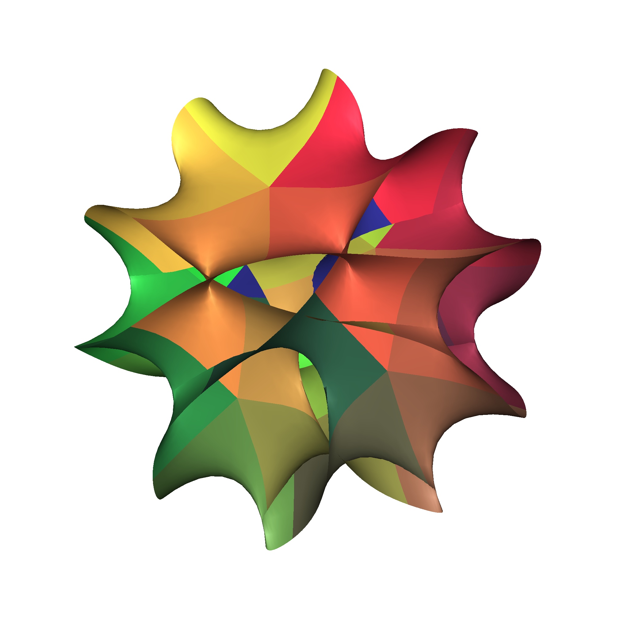
Lectures in January 2025 at the Simons Center for Geometry and Physics
Notes by Patrick Lei
WHAT’S A PUBLISHER?
Preface
These notes, taken during the first two weeks of the program Recent developments in higher genus curve counting at the Simons Center for Geometry and Physics, explain how to prove important structural results in the higher-genus Gromov-Witten theory of compact Calabi-Yau threefolds.
One of the oldest problems in Gromov-Witten theory is to compute the Gromov-Witten invariants of compact Calabi-Yau threefolds. While there are a variety of physical methods which have allowed physicists to make spectacular predictions in a wide range of examples, mathematical progress has often been frustratingly slow due to a lack of satisfactory tools to attack the problem with. To illustrate this, we will briefly outline some developments in mathematics regarding Calabi-Yau threefolds with which arise as complete intersections in weighted projective space.
For complete intersections in projective space, a genus-zero mirror theorem was proved by Givental in 1996 and Lian-Liu-Yau in 1997 [Giv96; LLY97]. For complete intersections in weighted projective space, a genus-zero mirror theorem was proved by Coates-Corti-Lee-Tseng in 2006 in the convex case and by Jun Wang in 2019 in the non-convex case [CCLT09; Wan20]. The main difficulty in the non-convex case is the failure of the quantum Lefschetz theorem [CG07], which is the main tool used in [Giv96; LLY97; CCLT09].
Meanwhile, a genus-one mirror theorem was proved for the quintic by Zinger in 2007 and for complete intersections in projective space by Popa in 2010 [Zin09; Pop13]. This used the theory of reduced invariants developed by Vakil-Zinger and Li-Zinger [VZ08; LZ09], which is a technique of performing birational modifications to the main component of the moduli space of stable maps to force the quantum Lefschetz theorem to hold so that computations can be performed using virtual localization [GP99]. Unfortunately, to this date no computations have been successfully performed using reduced invariants since.
Another approach is to consider the theory of GLSMs [Wit92], which were constructed mathematically by various authors [FJR18; FK21] during the 2010s. Unfortunately, the virtual cycle is supported on the moduli space of stable maps to the threefold, which does not carry a torus action. For the quintic, the ambient space of the relevant GLSM is the total space of . A standard way to gain a torus action is to compactify the moduli space at infinity and consider relative (or logarithmic) invariants. This leads to the theory of logarithmic GLSMs, which was introduced by Chen-Janda-Ruan in 2019 [CJR21]. Before this, Guo-Janda-Ruan used this theory [CJR23], including still conjectural foundational results [CJRa; CJRb], to prove a genus-two mirror theorem for the quintic in 2017 (up to the fact that the moduli space used in their 2017 paper is still not defined) and to prove the Yamaguchi-Yau finite generation conjecture, holomorphic anomaly equations, and orbifold regularity (as well as the conifold gap condition in low genus) for the quintic [GJR17; GJR18].
Because a GLSM is an enumerative theory of a critical locus in a GIT quotient, it depends on a stability parameter. We can vary the stability parameter and construct a master theory following the master space construction of Thaddeus [Tha96]. This leads to the theory of Mixed-Spin-P fields, which was first constructed by Chang-Li-Li-Liu in 2015 (for the quintic only) [CLLL19; CLLL22]. Unfortunately, the original theory is impossible to compute with when , so a parameter was introduced by Chang-Guo-Li-Li in 2018 [CGLL21]. In the same year, Chang-Guo-Li proved the Yamaguchi-Yau finite generation conjecture, BCOV Feynman rule, and holomorphic anomaly equations for the quintic threefold [CGL21; CGL19]. These results were generalized to hypersurfaces in weighted projective space by the author in 2024 [Lei24b; Lei24a], where a genus-one mirror theorem was also proved.
The Castelnuovo bound was proved in 2022 by Liu-Ruan [LR22] for any Calabi-Yau threefold satisfying a conjectural Bogomolov-Gieseker-type inequality (including the quintic) due to Bayer-Macri-Toda [BMT14] and a weaker version of the result was proved by Zhiyu Liu in 2024 [Liu24] without assuming the conjectural inequality. These results were obtained using the GW/DT correspondence [MNOP06a; MNOP06b], which was proved for complete intersections in products of projective spaces by Pandharipande-Pixton in 2012 [PP17] and for all Calabi-Yau threefolds by Pardon in 2023 [Par24].
As we can see, two major breakthroughs were made around the year 2018, when mathematicians discovered ways which make proving results about Gromov-Witten invariants in arbitrary genus tractable.1 These notes explain how to use these new ideas to prove the most important conjectures which are provided to us by physicists, namely the Yamaguchi-Yau finite generation conjecture and the holomorphic anomaly equations. Chapter 1 covers the B-model topological string and the Givental formalism, Chapter 2 covers log GLSMs, and Chapter 3 covers Mixed-Spin-P fields. We will cover both the foundational theory and the calculations in both approaches – in particular, Section 2.1 and Section 3.1 discuss the geometry of the log GLSM and MSP moduli spaces while Section 2.2 and Section 3.2 discuss calculations.
Author’s note
In contrast to the genus zero situation, not much is known about higher-genus Gromov-Witten theory. This is in part because there are significantly fewer tools to study higher-genus invariants, and the ones which do exist seem to be considered extremely inaccessible. It is my sincere hope that these notes can help make the subject more accessible.
All errors are the sole responsibility of the author. Please email me if you find any mistakes or typos in these notes.
The lectures were divided as in Table 1. The notes from the lectures by Albrecht Klemm were taken partly during the lecture and partly by watching the videos on the SCGP website, the notes from my lectures are slightly expanded versions of my lecture notes, and the notes from all other lectures were taken during the lecture, with some material being provided by the speakers after their lectures. All references were added after the lectures.
| Date | Time | Subject | Speaker(s) |
| 1/6/25 | 9:30 | Log GLSM foundations I | Qile Chen |
| 1/6/25 | 11:30 | Givental formalism I | Patrick Lei |
| 1/7/25 | 9:30 | Log GLSM foundations II | Qile Chen |
| 1/7/25 | 11:30 | Givental formalism II | Patrick Lei |
| 1/8/25 | 9:30 | Log GLSM foundations III | Qile Chen |
| 1/9/25 | 9:30 | Physics I | Albrecht Klemm |
| 1/9/25 | 11:30 | Log GLSM virtual localization | Felix Janda |
| 1/10/25 | 9:30 | Physics II | Albrecht Klemm |
| 1/13/25 | 9:30 | MSP moduli space: quintic | Wei-Ping Li |
| 1/13/25 | 11:30 | Genus two and LG/CY via log GLSM | Shuai Guo, Felix Janda |
| 1/14/25 | 9:30 | Polynomiality via MSP | Patrick Lei |
| 1/14/25 | 11:30 | GW theory of the quintic via log GLSM | Shuai Guo, Felix Janda |
| 1/15/25 | 9:30 | -stability I | Yang Zhou |
| 1/16/25 | 9:30 | -stability II | Yang Zhou |
| 1/17/25 | 9:30 | BCOV Feynman rule via MSP | Shuai Guo |
Acknowledgements
I would like to thank Qile Chen, Felix Janda, Sheldon Katz, Melissa Liu, John Pardon, and Rachel Webb for organizing the program. I would also like to thank Konstantin Aleshkin, Shuai Guo, Melissa Liu, and Dimitri Zvonkine for helpful discussions regarding the material in my lectures. Further thanks goes to Qile Chen for generously providing the notes from his lectures, Felix Janda for pointing out some subtleties and correcting some errors related to the material in his lectures, Sheldon Katz for pointing out that the Kähler structure bundle is the dual of the Hodge bundle, Yang Zhou for making detailed suggestions, and the Simons Center for posting videos of all of the lectures.
1 Mathematical and physical preliminaries
We begin these notes with discussion of the topological B-model. Using mirror symmetry, physicists are able to transport questions in Gromov-Witten theory (the A-model) to the B-model, which lacks a satisfactory mathematical definition. The benefit of doing this is that it is easier to calculate in the B-model, where genus-zero invariants are simply period integrals. Using other B-model techniques,1 physicists are able to make far-reaching predictions about the Gromov-Witten invariants of Calabi-Yau threefolds. Note that there are proposed mathematical definitions of the B-model – the analytic approach of Costello-Li [CL12b; Li11] and the categorical enumerative invariants of Caldararu-Tu [CT24] – but they are extremely difficult to compute with.
We then proceed to a discussion of the mathematical prerequisites for the calculations which appear later in these notes. The most important tool for performing calculations in Gromov-Witten theory is the formalism introduced by Givental in a highly influential series of papers [Giv01b; Giv01a; Giv04] in the early 2000s. This formalism allows us to package large formulae, for example coming from virtual localization, in a compact way, which allows us to reason about higher-genus invariants in a relatively streamlined way. For example, polynomiality of GW generating series will be a direct corollary of polynomiality of the entries of an -matrix which plays a central role in Givental’s formalism.
1.1 Introduction to the topological B-model
1.1.1 Mirror symmetry and the role of Calabi-Yau threefolds
Let be a Calabi-Yau -fold, where here is a holomorphic -form and is a Kähler form. Recall that this is equivalent to having holonomy or to . By a result of Yau [Yau78], there exists a Kähler-Einstein metric in the class of with vanishing Ricci curvature. For our purposes, we will mostly consider the case when .
We will really consider families of Calabi-Yau varieties
where is parametrized by a combination of complex structure moduli and Kähler structure moduli complexefied by a Neveu-Schwarz harmonic -form to . We will denote the fiber by
On the moduli of complex structures , the tangent space has a basis given by harmonic forms
for . Because we are in the Calabi-Yau setting, contracting with gives us a basis
of . By a theorem of Tian-Todorov [Tia87; Tod89], the moduli space is unobstructed. The B-model is built from mathematical structures on .
There is a moduli space 2 parameterized by subject to the condition
To first order, we have
The indices with pure Hodge type correspond to harmonic forms in with components
yielding the Kuranishi family over . The mixed indices correspond to real harmonic -forms, and expanding the Kähler form linearly we obtain
in terms of real Kähler parameters
which are volumes of holomorphic curves.
The Kähler moduli space is the real Kähler cone subject to positivity conditions from integration over -dimensional holomorphic submanifolds, namely
The bosonic part of the string action contains the harmonic antisymmetric Neveu-Schwarz background field
where is the string coupling constant. Its critical values measure complexified volumes of holomorphic curves by
Conjecture 1.1.1.
For non-rigid Calabi-Yau threefolds with , there exists a mirror Calabi-Yau with and such that the moduli spaces satisfy
and all relevant physical and mathematical structures can be identified using locally invertible mirror maps
Mirror symmetry identifies Type IIA compactifications on with Type IIB compactifications on , and vice versa. Additional Ramond-Ramond background fields and axio-dilaton fields with modulus and extend the moduli spaces as
and
where denotes a quaternionic extension of . The RR -form fields are sourced from branes. is even for Type IIA and odd for Type IIB. The correspond to coherent sheaves and correspond to special Lagrangian branes. Here, is the d hyper-multiplet moduli space, and is the d vector multiplet moduli space.
One kind of mathematical structure is Hodge numbers. In the traditional picture of the Hodge diamond, Poincaré duality corresponds to a reflection along the horizontal axis, Dolbeaut symmetry is a reflection along the vertical axis, and mirror symmetry is a reflection along a line with slope .
Superstring theory is defined by maps
weighted by an action which is a supersymmetric extension of the area of . It is easy to quantize the Neveu-Schwarz-Ramond action, and the Green-Schwarz action incorporates the RR fields. The first quantized theory is defined by a variatonal integral with partition function
Superstring theory is Weyl invariant in ten dimensions, or in other words
so we obtain a discrete sum of finite-dimensional integrals. This implies that the compact part of the spacetime must be a complex threefold. If is Calabi-Yau, we obtain an extended world-sheet SCFT, which has four nilpotent operators
The -twist corresponds to taking
and the -twist corresponds to
The topological -model yields a cohomological topological theory depending only on the Kähler structure, while the topological -model is a homological topological theory depending only on the complex structure. Mirror symmetry then exchanges the -model and -model.
1.1.2 The topological A-model and B-model
In the -model, terms depending on the complex structure are -exact, so the variatinoal integral simplifies to
Here, we have
and these holomorphic maps are stationary points of the action. Moreover, taking the logarithm, we obtain
where are the GW invariants. Rewriting these in terms of GV invariants, we obtain
In the -model, the terms depending on the Kähler structure are -exact and the variational integral localizes to constant maps albeit with a nontrivial measure depending on the complex structure. Mirror symmetry is supposed to be an exact duality, so we should have
Period integrals
define a nondegenerate pairing between middle homology and cohomology by Stokes’ theorem. This pairing is antisymmetric if is odd and symmetric if is even. For example, if is a K3 surface, then the lattice is
If is odd, we can fix an integral symplectic basis , which is defined only up to the action of .
Example 1.1.2.
If we consider an elliptic curve , then we obtain
and
Then the integrals
are elliptic integrals. The periods are annihilated by the Picard-Fuchs operator, and by definition thus satisfy the equation
The main constraints which govern the periods of a Calabi-Yau -fold are the Riemann bilinear relations
This defines the exponential of the Kähler potential for the Weil-Petersson metric
on . There are also holomorphic bilinear relations
which follow from Griffiths transversality [Gri68a; Gri68b]. Here, the integrand in the left hand side are arbitrary combinations of derivatives of with respect to the . We will see later that these give rise to propagators, the holomorphic anomaly equations, and other structures. The are rational functions labelled by up to permutations.They are also determined by differential ideals also determine the up to normalization.
Remark 1.1.3.
In terms of the periods , if we write them in a basis compatible with the intersection form , the quantities in the relations may be written as
1.1.3 The quintic
Consider the mirror quintic , which is given by the equation
The period vector (with an appropriate choice of integral cycles) fulfills the Picard-Fuchs equation
where .
We want to find a basis where the monodromies around the singular points are integral symplectic matrices, so we look at the Riemann symbol and see that it is given by
Here, is a point of maximal unipotent monodromy, is the orbifold (or Landau/Ginzburg, or Gepner) point, and is the conifold point. At a point of maximal unipotent monodromy, we can expand the mirror map and go to the large volume limit point in the -model.
Using special geometry, Bryant and Griffiths [BG83] showed that the periods may actually be expressed using a prepotential as
These correspond to triple logarithmic, double logarithmic, analytic, and logarithmic solutions, respectively. Using this, we can make the identification
where the mirror map is given by
This was generalized to multi-parameter models by Hosono et. al [HKTY95], who related the classical terms to CTC Wall data and in the formula
Later, we will use this to find the integral symplectic basis without calculating any monodromy.
We now turn our attention to calculating the numbers . We already saw the genus-zero invariants, but we are also interested in the higher-genus ones. Some invariants in low genus and degree are given in Table 1.1.
Predictions were made by Candelas et al. [COGP92] for , Bershadsky et al. [BCOV94] for , and Huang et al. [HKQ09] for . The numbers , , and were calculated mathematically by Schubert, Katz [Kat86], and Ellingsrud-Strømme [ES96], respectively. Kontsevich [Kon95] gave a mathematical proof of some numbers in before the genus-zero invariants were completely determined by Givental and Lian-Liu-Yau [Giv96; LLY97]. The formula for the genus-one invariants was proved by Zinger [Zin09].
1.1.4 Fourteen one-parameter hypergeometric families
There are fourteen hypergeometric Picard-Fuchs operators for one-parameter families of Calabi-Yau threefolds given by
where the values of and are given in Table 1.2.
| Mirror | ||||||
|---|---|---|---|---|---|---|
Here, the notation for the mirror means the complete intersection in the weighted projective space with weights given in parentheses with degrees given by the subscripts. The local exponents are all at the MUM point, at the conifold point , and are given by at the orbifold point . The monodromy around a singular point is captured by the minimal exponent3 such that
for some . When and , then we have an orbifold point. When we have an infinite shift monodromy. If and the local exponents take the form , then we have a single vanishing period dual to a logarithmic degenerating period and hence a conifold point, and if the local exponents are take the form , then we have two vanishing periods and two logarithmic degenerating periods, and this case is called a -point. The case cannot occur by Schmid’s orbit theorem, and when , we have a point of maximal unipotent monodromy with local exponents .
At the point , there is a Frobenius basis of solutions
where we normalize the power series to have and . Therefore, we can find an integral basis
In the integral basis, all monodromies are integral symplectic matrices. At the point , we have
and at the conifold point, we have
At , we have .
The work of Alexandrov-Feyzbakhsh-Klemm-Pioline-Schimannek [Ale+24] solves the topological string on these models up to given in Table 1.3 using brane and wall-crossing.4 Note that is the maximum genus for which data appears at http://www.th.physik.uni-bonn.de/groups/klemm/data.php and is the maximum genus solved by the work of Huang-Klemm-Quackenbush [HKQ09].
| Type | |||||||
|---|---|---|---|---|---|---|---|
Remark 1.1.4.
Even inserting at least one brane requires going beyond the topological string, which only gives the usual DT or PT invariants (one brane, no branes, and arbitrary and brane charges). Hopefully, we will be able to explore the entire space of Bridgeland stability conditions in the future.
1.1.5 More on periods
Consider the Picard-Fuchs operator
of a one-parameter Calabi-Yau -fold with middle Hodge structure of type . Defining the adjoint operator
then Griffiths transversality implies that the operator is essentially self-adjoint, or in other words
Here, the Yukawa coupling satisfies the differential equation
For the quintic, we in fact obtain
Equivalently, self-adjointness implies
When , this yields
In the multi-parameter case, the periods span the kernel of the Picard-Fuchs differential ideal
generated by the differential operators
This system is complete if all three-point functions
can be integrated from the Griffiths transversality relations.
Example 1.1.5.
For the example with middle Hodge structure , the Picard-Fuchs equation is generated by
and the are given by
where the components of the discriminant are given by
and .
If we shift the holomorphic form by
this induces a Kähler gauge transformation
Also note that the Yukawa couplings are sections of
where is the dual of the Hodge bundle.
By the local Torelli theorem [Gri68a; Gri68b], the components of the period vector
are homogeneous coordinates on . Griffiths transversality implies that
is a homogeneous prepotential such that
and the Yukawa couplings are given by
Dividing by , we will get inhomogeneous coordinates , and we obtain the inhomogeneous prepotential
The Kähler potential and Yukawa coupling become
In addition, we have
In inhomogeneous coordinates, we can obtain the period vector from by
The Picard-Fuchs equation is equivalent to the Gauss-Manin connection
where and . If we set
this becomes
1.1.6 Special geometry
On the moduli space of complex structures , we have metric connections from the Weil-Petersson metric and the Kähler line bundle connection. On sections
the covariant derivatives are given by
Using the covariant derivatives, we see that and .
Proceeding more systematically, repeated applications of yield
Using the relation
we further deduce
It follows that
where . This equation is known as the special geometry equation and is the integrability condition for the existence of the prepotential .
1.1.7 Genus one predictions
In a theory, the topological torus partition function is defined by
as an integral of the fermion number projected partition function over the fundamental region of the torus. Using its relationship to the family index of Ray-Singer analytic torsion [FLY08], it satisfies the holomorphic anomaly equation
Using and the special geometry equation, we can integrate the holomorphic anomaly equation to obtain
| (1.1) |
1.1.8 Propagators
The propagators are an-holomorphic sections , , and of , , and , respectively, defined by
We can integrate the first equation using the special geometry equation and the observation that the only contributions to are derivatives in . Therefore, if there exists an index such that is invertible, we obtain
where is the holomorphic propagator ambiguity.
Following Alim-Länge [AL07], it is convenient to shift the remaining propagators as
Applying the special geometry equation, we obtain
Here, all of the ambiguities are in fact rational functions in with rational coefficients. This allows us to obtain explicit formulae
Taking the holomorphic limit of the propagators, we obtain
where we take the holomorphic limits , , and .
Returning to the genus one situation, the holomorphic anomaly equation becomes
where we define . This can be integrated to obtain Equation 1.1. The holomorphic limit is given by
where the holomorphic ambiguity is given by
1.1.9 Higher-genus predictions
In higher genus, the holomorphic anomaly equation becomes
This can be rewritten as the system of equations
assuming that , , , and are algebraically independent. Using the shifted propagators, we obtain and
Using the method of direct integration, due to Yamaguchi-Yau, Grimm-Klemm-Mariño-Weiss, and Alim-Länge [YY04; GKMW07; AL07], we obtain
Here, we set
Therefore, we can solve for a polynomial , which is a weighted polynomial of degree with the weights . For example, in the one-parameter case, we obtain
1.1.10 Boundary conditions
The most difficult part of computing is the degree-zero part , which is known as the holomorphic or modular ambiguity. In the hypergeometric cases, we have
where the number depends on the type of singularity at . At , the boundary conditions come from the asymptotics
The second equality uses the computation of degree-zero GW invariants by Faber-Pandharipande.
In the one-parameter case, the Castelnuovo bound implies that the GV invariants are nonzero only when the genus is strictly less than in general and when . This was first observed by Huang-Klemm-Quackenbush [HKQ09] and proved in 2023 by Feyzbakhsh (in the paper [Ale+24] of Alexandrov et. al). Because curves of degree of genus are smooth, the associated invariants may be obtained by the formula
where denotes the deformation space of the curve. For the one-parameter hypergeometric cases, we obtain
The most important boundary condition is the gap condition at the conifold point , where a -cycle with the topology of a lens space vanishes. Here, this says that we have
for all , where is the local coordinate at the conifold point given by the ratio of a vanishing and non-vanishing period.
1.2 An axiomatic approach to enumerative geometry
1.2.1 Moduli of curves and CohFTs
We will denote by the moduli space of stable curves of genus with marked points. This is nonempty if and only if , in which case it is a Deligne-Mumford stack of dimension . There is a combinatorial structure to the collection of , which is given by a collection of morphisms.
- •
There is the gluing morphism
which takes two curves and glues them along the last marked point to form a node;
- •
There is the self-gluing morphism
which glues the last two marked points.
There is of course another interesting map, which is the forgetful map
given by deleting the last marked point and then stabilizing. We are now able to define our enumerative theories of interest, which include Gromov-Witten theory.
Definition 1.2.1.
Given a vector space with a nondegenerate symmetric bilinear form and a unit element , a Cohomological Field Theory (CohFT) [KM94] on is a collection of -equivariant linear maps
which satisfy the basic identity
and the following combinatorial identities (we will let be a basis of such that and be the dual basis):
If in addition the identity
is satisfied, then we say the CohFT has a flat unit (or satisfies the string equation).
All of this can be generalized to super vector spaces, but for simplicity we will not deal with this case.
Example 1.2.2.
The most important example of a CohFT is the Gromov-Witten theory of a smooth projective variety . Here, recall that the source of a stable map is a prestable curve, so there is a stabilization morphism
which forgets the map and stabilizes the curve. Then, working over the Novikov ring, we will set , to be the Poincaré pairing, and to be the fundamental class of . The linear maps are given by the formulae
where is the -th evaluation map.
Example 1.2.3.
Let be the universal curve. Then the Hodge bundle is the vector bundle
We then consider the vector space with the usual pairing and define the CohFT by the formula
The gluing axioms are satisfied by the equation and the exact sequence
Here, because genus zero components do not contribute to global sections of and does not depend on the marked points, this CohFT has a flat unit.
Remark 1.2.4.
We will see later that this is related to the GW CohFT of a point by the quantum Riemann-Roch theorem [CG07].
Given a CohFT , we may produce invariants by pairing the classes with various cohomology classes on . The most important ones to consider are the classes
where is the -th marked point.
Remark 1.2.5.
In Gromov-Witten theory, these are called ancestors. There are also descendants, which are given by the same formula except using the moduli space of prestable curves instead of , where we factor the morphism defined above as
The descendant classes are denoted by .
Example 1.2.6.
We will calculate an invariant which will appear in the GW theory of Calabi-Yau threefolds. For any CohFT , consider the invariant
Using the second gluing equation, the degree zero part of is equal to
which yields the (graded) dimension of . Therefore, we obtain
Example 1.2.7.
Consider the GW CohFT of a point. This is given by with the usual pairing and the formula
Then we define the invariants
Theorem 1.2.8 ([Kon92]).
The function
is annihilated by the operators
Remark 1.2.9.
This result (Virasoro constraints for a point) is equivalent to being a tau-function for the KdV hierarchy and has been generalized by various authors.
1.2.2 The genus-zero picture
A CohFT in genus zero defines a Frobenius manifold [Dub96]. In particular, there is a product structure defined by the formula
and the quantum connection, which is defined by the formula
The structure of a Frobenius manifold comes from a function , which is known as the genus-zero descendant potential and satisfies a set of PDEs, which are the string equation, dilaton equation, and an infinite set of topological recursion relations, where we write :
To state the following result, we consider the infinite-dimensional vector space (or a completion of this) with the symplectic form
We also consider the new variable5 , so is now a function near .
Theorem 1.2.10 ([Giv04]).
satisfies the above PDEs if and only if the graph of is a Lagrangian cone with vertex at such that its tangent spaces are tangent to exactly along .
We may recover the Lagrangian cone by the following procedure. We find a fundamental solution
to the quantum connection, which satisfies the equation
Then, setting , we can then recover the Lagrangian cone by the following procedure:
- •
The derivatives form a basis of ;
- •
This implies that . Writing these in terms of the first derivatives and using the fact that solves the quantum connection, we recover the Frobenius structure and hence the Lagrangian cone.
In Gromov-Witten theory, there is an explicit formula for the fundamental solution in terms of descendant invariants. It is given by
Example 1.2.11.
Let be the quintic threefold. We will use the genus-zero mirror theorem of Givental to compute the quantum product on . Let
be the (very small) -function of . Setting , the mirror theorem states that
Because the mirror map corresponds to setting by the divisor equation, we can use the mirror theorem to compute . Because of our nonstandard choice of the -function, the quantum connection becomes the ODE
where (here, the coordinate is ) and . An explicit computation using the mirror theorem and the results of Zagier-Zinger [ZZ08] yields
Because begins with the identity, this computes .
1.2.3 -matrix action
In the early 2000s, Givental [Giv01a; Giv04] discovered a remarkable property of axiomatic enumerative theories, namely that one can transform CohFTs by the action of matrices which satisfy the property
Traditionally, the literature [PPZ15] requires that and , but the MSP group [CGL19] has removed this restriction and also allows .
In order to define the action of on a CohFT defined on , we need to review some of the combinatorial structure of . For a curve , we may consider the dual graph of , which has vertices, edges, and legs, which are defined as follows:
- •
The vertices correspond to irreducible components of and are labelled by a non-negative integer, which is the genus;
- •
The edges correspond to nodes of (in particular, we allow loops);
- •
The legs correspond to marked points.
Any graph which appears as the dual graph of a stable curve is called a stable graph.
The first type of action on CohFTs is a translation action. Let . For a CohFT , we define
whenever the infinite sum makes sense.
Example 1.2.12.
If is the GW CohFT of a smooth projective variety and is a divisor class, then the infinite sum makes sense and we can define the shifted GW CohFT of . For example, if is the quintic threefold and , then shifting to is the same as the mirror map .
The second type of action is the action of a matrix as in the beginning of this section. Let define the set of all stable graphs of genus with legs. Then we define
where is defined by the following construction:
- •
At the -th leg, we place the map
- •
At every edge, we place the bivector
- •
At every vertex, we place the linear map
- •
Finally, we consider the pushforward in cohomology along the gluing morphism
Definition 1.2.13.
Let be as above. Then we define the translation
Whenever it makes sense, we define
Theorem 1.2.14 ([CGL19]).
Suppose we work with coefficients in . Then if
is a well-defined CohFT. Moreover, if , is a unit for .
We would like to remark a bit more about the translation action when . For simplicity, we will assume that and for some constant . Then we set and use the dilaton equation to compute
whenever this makes sense.
1.2.4 Reconstruction theorem
Recall that every CohFT defines a Frobenius algebra. We will call a CohFT semisimple if the corresponding Frobenius algebra is semisimple.
Theorem 1.2.15 ([Tel12]).
Let be a semisimple CohFT with flat unit and be its topological part. If is semisimple, there exists a unique
such that
Example 1.2.16.
Recall the Hodge bundle CohFT from before. Recall that it is given by the formula
Taking the degree zero part, we see that is the GW CohFT of a point. Using Mumford’s computation
where , are the Bernoulli numbers, and is the inclusion of the boundary up to a étale cover, and the formula
for any vector bundle (or by just using the quantum Riemann-Roch theorem6 directly), we obtain the -matrix
As a sanity check, we will compute using the -matrix. First, we consider the stable graphs in Figure 1.2.
The first graph gives us the contribution
Using the formula and the fact that , this becomes
The second graph does not receive tail contributions because . The constant term of the edge contribution is , so considering the automorphism and pushing forward to gives us
where denotes the boundary divisor (with the correct stack structure). Because in this case, we obtain
1.2.5 Operator formalism and geometric quantization
We will return to the symplectic formalism of Givental. This is more convenient for certain computations, but it is in fact equal to what we have before, at least when we want to calculate generating functions. Recall that we had a Frobenius manifold structure on and we considered the vector space with symplectic form
If we consider the polarization given by and , then letting be as before (with the dilaton shift), let be coordinates on such that form a system of Darboux coordinates for .
Definition 1.2.17.
We will call any formal function of the form
an asymptotic element of the Fock space.
Then given such an asymptotic element of the Fock space, we will quantize (infinitesimal) symplectic transformations on by the following formulae:
In particular, this will allow us to understand expressions like . However, we need to be careful because our formulae will involve both the fundamental solution and the -matrix, and is a power series in .7
Theorem 1.2.18 ([Giv01a]).
An operator of the form acts on (asymptotic) elements of the Fock space by the formula
where is defined by the formula
Operators of the form act by the formula
where is defined by
For a semisimple CohFT, there is a system of canonical coordinates such that the -form is a homomorphism of algebras . Then near a semisimple point, there is a asymptotic solution to the quantum connection of the form
where switches from flat coordinates to canonical coordinates and is the matrix of canonical coordinates. Finally, define
A corollary of Teleman’s reconstruction theorem is the formula
for the Gromov-Witten theory of any smooth projective variety with semisimple quantum cohomology.
Example 1.2.19.
As a final example, we will apply Teleman’s theorem to compute of any semisimple CohFT. This result was first proved by Givental [Giv98] for the equivariant Gromov-Witten theory of GKM orbifolds and extended to the orbifold case by Zong [Zon16]. The argument we give is due to Guo-Ross [GR19]. Let denote an idempotent basis for the quantum product. We will compute
Using the reconstruction theorem, we obtain
Using the identities
| (1.2) | ||||
where , we obtain the result
which can be placed in the suggestive form
We will now prove the identities in Equation 1.2. For the first identity, we will compute using the reconstruction theorem. There are two stable graphs, given in Figure 1.3.
The first graph gives the contribution
The second graph gives the contribution
This has multiplicity , so taking the sum and integrating over , we obtain
where we have used the fact that
This proves the first identity.
To prove the second equality in Equation 1.2, we note that
because is idempotent. Differentiating with respect to , we obtain
Using again the fact that is idempotent, we see that
This implies that
which proves the identity.
2 Higher-genus computations via log GLSM
In algebraic geometry, one profitable way to deal with non-compactness issues is to forcibly compactify our spaces and then understand the contributions coming from the divisor at infinity. For example, this technique was used by Deligne to construct mixed Hodge structures [Del71]. In enumerative geometry, one profitable application of this technique is the capped topological vertex [OP10], which calculates relative invariants of a (partial compactification) of relative to the divisor at infinity and is related to the usual topological vertex by a capping operator. While Jun Li’s technique of expanded degenerations [Li01] allows us to calculate enumerative invariants relative to a smooth divisor, generalizing this to the case of a simple normal crossings divisor requires logarithmic geometry (at least if we want to do it using algebraic geometry). Now, Chen-Janda-Ruan [CJR21] have developed the theory of log GLSMs, which define stable map-type invariants for any GLSM-type theory defined over an arbitrary projective Deligne-Mumford stack (and resolves all compactness issues therein). This theory has been used by Guo-Janda-Ruan [GJR18] to prove finite generation, holomorphic anomaly equations, orbifold regularity, and the LG/CY correspondence for the quintic threefold and some other Calabi-Yau threefold complete intersections in projective space.
2.1 Geometry of log GLSM moduli spaces
Our motivation is the quantum Lefschetz theorem. Here, we let be a smooth projective variety or Deligne-Mumford stack over and be a vector bundle over . We are interested in computing the Gromov-Witten invariants of a smooth complete intersection defined by a regular section of . Because the ambient space is generally easier to work with, it is desirable to find a way to compute the GW invariants of in terms of the data of .
Question 2.1.1.
Is there a way to compute the Gromov-Witten invariants of using the ambient data of , possibly involving some correction terms?
While quantum Lefschetz holds in genus zero in the convex case, and the approach of desingularization of the moduli of stable maps to force quantum Lefschetz to hold works well in genus one, this is intractable in higher-genus. Instead, our approach will be to use GLSMs, which were introduced by Witten [Wit92] in the physics literature, and by Fan-Jarvis-Ruan and Kiem-Li, Chang-Li, Chang-Li-Li, and other authors in mathematics [FJR18; KL13; CL12a; CLL15]. We will combine this with the theory of punctured log maps due to Abramovich-Chen-Gross-Siebert [ACGS24] to obtain the theory of log GLSM.
2.1.1 -maps and log targets
Definition 2.1.2.
An -map is a commutative diagram
where the morphism is a proper, log-smooth DM-type morphism. If the source is a twisted curve, this is the underlying -map. If the source is a log curve, this is a log -map, and if the source is a punctured curve, this is a punctured -map.
Example 2.1.3.
Consider the diagram
Taking the base change of the underlying -map to , consider the diagram
Therefore, the data of an -map to this target is equivalent to the data of a morphism and a section . In particular, if , we are left with the data of a differential .
Example 2.1.4.
We will now give some examples of some log targets. An easy way to compactify a vector bundle is to turn it into a weighted projective space bundle, so for example we may consider
We can give this the log structure of functions which vanish only on the boundary and call it .
Another example is to consider the example of -spin curves. Here, with the degree map to . Then we set
Again, we give this the divisorial log structure and call it .
A feature of this is that there is a geometric LG/CY correspondence, namely that as log stacks.
Example 2.1.5.
For the complete intersection in , we consider
with the divisorial log structure.
Example 2.1.6.
We will now consider a general hybrid target. The input is a smooth projective DM stack , a vector bundle over , a line bundle over , and . The spin is the diagram
The target is
with the divisorial log structure at infinity.
We will now turn our discussion to the discrete data. This consists of a genus, curve class, and twisted sector for each marking. We will now construct a dual graph, which has vertices and half-edges. There is an involution
and a vertex map . Legs are the half-edges which are fixed by the involution, and we will label the legs by the marking map
The decorations are the curve classes, sectors, and degrees.
Consider a log map
where is a special point. Because is the trivial bundle, we obtain a commutative diagram
which exhibits as a gerbe over . Assuming that there are no orbifold points, theere is a sector map
We require that factors through , and say that is compact type if .
Example 2.1.7.
Consider again . Then . If , then a log map is simply , which cannot be stable. Adding a marked point, we obtain a section of , which we will force to vanish at the marked point.
The stability of underlying -maps has two conditions:
- 1.
First, that the morphism is representable;
- 2.
Second, that
where is a polarization on the target. Here, .
Example 2.1.8.
Again considering , we will let be of genus . the limit is the union of a genus-zero curve with a differential which vanishes at one point with multiplicity connected to a genus curve which sits entirely at infinity. Even though the rational component is not a priori stable, it is stabilized by its intersection with the zero section.
Remark 2.1.9.
In the case, stability is equivalent to the condition that
whenever .
2.1.2 Log geometry and tropicalization
Definition 2.1.10.
Let be a scheme or a stack. A log structure on is a sheaf of monoids on , together with a morphism
inducing an isomorphism . The pair is called a log scheme/stack and the sheaf
is called the characteristic sheaf or ghost sheaf.
Example 2.1.11.
Any log GLSM target is a log stack.
Example 2.1.12.
Another standard target is a toric variety with being all functions which vanish only on the toric boundary. This is usually called the divisorial log structure.
Example 2.1.13.
For a toric monoid , we can consider
The tropical data we will consider is the category of rational polyhedral cones . This has a distinguished object . Locally, we will define
with the natural lattice structure . In general, the tropicalization of a log scheme is the generalized cone complex given by gluing local pictures along face maps.
Example 2.1.14.
Consider with the log structure given by . Then
Here, there is only a log structure at , which is a copy of measuring the vanishing order at the origin. The map
sends to , so induces .
Example 2.1.15.
Consider with the toric log structure. Then is simply , which is the same as the support of the toric fan. At the monoid level, there is an at the origin, a copy of on each axis, and at a general point.
2.1.3 Log curves
Definition 2.1.16.
An -pointed log curve over a log scheme consists of
such that
- 1.
The underlying morphism of is an -pointed twisted curve;
- 2.
is log smooth and integral;
- 3.
On the smooth locus of , the log structure is given by
Intuitively, the log structure is given by the log structure at smooth unmarked points, at marked points, and at the nodes, which means the pushout diagram
Here, is the edge length parameter, and and are the two components.
Because tropicalization is functorial, the morphism induces a morphism
For example, if has two components, then the node will correspond to the largest cone, each component corresponds to a copy of , and each marking will give a leg of infinite length. Above a point in , the distance between the two components is the edge length parameter evaluated at the point . To see this more clearly, see Figure 2.1.
We will now consider punctured curves. We will consider a diagram
Here, is a morphism of log schemes which is an isomorphism away from and is an isomorphism. In addition, we will have an inclusion
This corresponds to allowing poles at , and in the tropicalization makes edges finite-length. A picture is given in Figure 2.2.
Definition 2.1.17.
A punctured curve is a log curve with punctures
A tropical punctured curve is a tropical curve with the additional data of lengths of punctured legs.
2.1.4 Superpotentials
Definition 2.1.18.
A superpotential is a commutative diagram
where . We say that has proper critical locus if
is proper.
Equivalently, a superpotential is a -equivariant function
In this formulation, has proper critical locus if and only if is proper (as a DM stack). This implies that the critical locus is contained in .
Example 2.1.19.
Let be a smooth projective Deligne-Mumford stack and be a vector bundle on with section . We will write
Then is proper if and only if is smooth of codimension equal to the rank of .
Example 2.1.20.
Let and . Let be nonzero. Now is simply multiplication by , so the critical locus is empty.
2.1.5 Punctured -maps
Definition 2.1.21.
A punctured -map is an -map with domain a punctured -map.
Definition 2.1.22.
Let be a half-edge. Then the contact order at is defined by
Example 2.1.23.
Consider the genus picture from before (target being ) and consider the same stable limit as an -map. If we calculate with , then
so the pole order at the node must be . Tropically, if is the half edge of the node attached to the vertex, we have , so restricting to the component, we obtain a punctured -map.
The discrete data of punctured -maps is
Theorem 2.1.24.
The moduli stack is a proper log DM stack admitting a canonical perfect obstruction theory.
Definition 2.1.25.
We will consider where and . These are called vertex-type moduli. If , then we will denote
for the stack of stable log -maps, and if , the we will denote
for the stack of punctured -maps.
2.1.6 Obstruction theories
Definition 2.1.26.
Recall that we have a diagram
The canonical perfect obstruction theory is defined by
Because it is very complicated, we will not discuss .
Unfortunately, this is not the obstruction theory that we really want. We will consider the superpotential and then use the cosection localization technique of Kiem-Li [KL13]. Here, we have the diagram
whenever is of compact type. The compact-type condition implies that
factors through the sheaf of holomorphic differentials. Because , we obtain a cosection
By the results of Kiem-Li, this gives us a virtual cycle
supported on -maps to , which coincides with the canonical virtual cycle after pushing forward to the stack of all -maps.
Remark 2.1.27.
Of course, we have the problem that is not proper, so we need to find a way to extend the cosection along the boundary
We need to understand how to differentiate
which will require compact-type legs and a principalization of the boundary.
Definition 2.1.28.
We will say discrete data is compact type if for all , either
- •
and ;
- •
. In this case .
Example 2.1.29.
Consider the example in genus . If we consider , we can view it as . Then, at the marking, we see that and , so the leg is of compact type. In the tropical picture, the entire infinite leg gets contracted to the origin.
Example 2.1.30.
Now consider the same example but with . We will impose that there are no markings by . The stable limit as we scale to infinity had a genus component with a zero of order and a genus component mapping entirely to . If we consider the half-edge emerging from the genus vertex, it touches with contact order , so it is not compact type. On the other hand, the half-edge coming from the genus vertex touches with contact order , so it is compact type (and in the tropical picture the leg has finite length).
Remark 2.1.31.
The data of is equivalent to a fixed isomorphism , where is the genus vertex.
Remark 2.1.32.
Tropical curves with only compact-type legs have compact image in . In this picture, they are either pointing downward or contracted to the origin.
Having defined compact type insertions, we will now define a modular principalization of the boundary. There is an edge length
and a degeneracy
which intuitively records where is sent in .
Definition 2.1.33.
For a toric monoid , define a partial order if there exists such that . If we consider a punctured -map, consider the collection of degeneracies
It has uniform maximal degeneracy if there is a unique maximum
Example 2.1.34.
Let . Suppose that there are and a vertex which is sent to . Then we compute
Similarly, , where and are the generators of . These cannot be compared, so we do not have uniform maximal degeneracy.
To uniformize this, we consider a subdivision into three subcones. The first is when , the second is when , and the third is when . After this subdivision, each subcone has uniform maximal degeneracy.
Example 2.1.35.
A family of tropical curves over with compact-type legs and uniform maximal degeneracy has images in uniformly bounded from above by .
We now define a new stack
to be the stack of punctured -maps with discrete data and having uniform maximal degeneracy. By removing the condition of uniform maximal degeneracy, we obtain a morphism
which satisfies the following:
- •
is log étale, proper, and surjective;
- •
There is as canonical perfect obstruction theory;
- •
We have
for vertex-type moduli.
The boundary defined by the Cartesian diagram
is a log Cartier divisor.
Theorem 2.1.36.
Assume all legs are of compact type and has proper critical locus. Then
- 1.
has a reduced perfect obstruction theory;
- 2.
In the log -map case, we have
- 3.
The boundary also has a reduced perfect obstruction theory;
- 4.
There is the relation
where is the pole order of at infinity.
The reduced perfect obstruction theory for log -maps is given by the triangle
and for is given by
The virtual components of are given by the formula
due to Abramovich-Chen-Gross-Siebert [ACGS24], where
is the tropical type of rigid tropical curves with uniform maximal degeneracy. Here, this implies that is bipartite and rigidity means there is no deformation fixing and besides scaling
Decomposing this further, we have
This is not true if we replace everything with the canonical obstruction theory, so this is quite interesting. Putting these two formulae together, we obtain the tropical decomposition formula
Example 2.1.37.
Consider the example again. When , we obtain six bipartite graphs, which are given in Figure 2.4.
Choosing any nonzero superpotential, we obtain the tropical decomposition formula
Note here that the critical locus is empty, so the virtual cycle must be zero.
In GW theory, the tropical decomposition formula becomes
2.1.7 Effective invariants
We will consider the reduced virtual cycle . For each , the evaluation lands in . Then effective invariants are given by
Remark 2.1.38.
In the vertex case, we have the relation
Before we continue, we will consider the geometry of when . Consider the diagram
This induces a stable map , so in fact it is equivalent to the data of and an isomorphism
which is equivalent to an isomorphism
Therefore, when , is the moduli of canonical divisors with specified zero orders, and for general , we have the moduli of -spin linear series of rank .
We can now take a root of the log target , which is given by the diagram
On virtual cycles, we obtain
where is either “vir” or “red.”
Geometrically, we must have a balancing condition
Example 2.1.39.
Let and suppose is a line bundle. Then we obtain
This implies that
so must be one of .
When , the upper bound is negative, so there are no genus zero reduced invariants. When , then the upper bound is zero, so the only reduced invariant is in the case . This implies that
so because the contact orders are all negative, they must equal .
Example 2.1.40.
We will consider legs of contact order in the case. Let be smooth of genus and . We now choose a marking , we obtain . The stable limit as we scale to infinity is a genus component mapping entirely to and a genus component with a zero at . On , we see that
This implies the contact order of the genus component with is , so the genus component has contact order .
Remark 2.1.41.
The legs with contact order are created by adding compact type markings outside of and should be viewed as the unit, denoted by .
2.1.8 Log GLSM axioms
Consider the diagram
where is the universal punctured curve.
Theorem 2.1.42.
We have the equations
and
for any . In addition, if we consider the diagram
then we have
Example 2.1.43.
If we consider and let , then we only need to compute one non-ambient invariant.
The reduced virtual dimension of is given by the formula
which also happens to equal
Therefore, when the virtual dimension of the stable map moduli is negative, then the reduced virtual dimension is zero.
Example 2.1.44.
Consider . The reduced dimension of is simply
We can remove all legs of contact order , so we reduce to the case when for all . Therefore, there are exactly reduced invariants.
Example 2.1.45.
For a general semi-positive hypersurface in , the reduced virtual dimension when is
Using the balancing condition, we obtain an upper bound of
If is negative, then the reduced virtual dimension is structly less than
After removing all legs of contact order , all effective cycles vanish! For example, we have this negativity whenever and , when and , and when and . For complete intersections in other targets, we can run the same arguments, and they are governed by birational invariants.
2.1.9 Uniform minimal degeneracy
Definition 2.1.46.
A punctured -map has uniform minimal degeneracy if there exists a unique
Sometimes, we will also need to consider disconnected graphs, so if we enforce uniform minimal degeneracy, we will obtain a cartesian diagram
where both vertical arrows are log blowups and hence log étale and projective. These introduce two new tautological classes on , which are
coming from and
coming from . The class is a key ingredient for the tropical decomposition and is needed for the virtual localization formula.
2.1.10 Some examples
Here, we will give a few exmples.
Example 2.1.47 (Quintic).
Here, the target is . We will consider the log target
with the infinity part
Example 2.1.48 (Double cubic).
Here, the target is . We will consider the log target
with the infinity part
Example 2.1.49 (Quintic FJRW).
We will consider the log target
with the infinity part
2.1.11 action
Our goal is now to proceed towards a virtual localization formula for log GLSM. Here, the two structural formulae are related as in Figure 2.5.
There are two ways to think about this -action. If we have an -map
this was a morphism of stacks, so there is a -morphism making the diagram commute. Abstractly, the action simply scales the -morphism, which is an isomorphism of line bundles.
More concretely, consider the quintic example. Then an -map is equivalent to the data of a stable map and a section of the projective bundle
Using this description, the -action simply scales the -field, where we scale the first summand and not the second.
We now have a action on all moduli spaces that we considered previously, for example or .
Proposition 2.1.50.
The perfect obstruction theories and are -equivariant.
Remark 2.1.51.
A key input to this result is that the superpotential is -equivariant. If it was in fact invariant, then there would be no need to develop the theory of log GLSM.
2.1.12 Fixed loci
There are several kinds of fixed loci:
- •
There is a fixed locus of all maps going into the zero-section.
- •
There is another fixed locus of maps going into infinity.
- •
More general fixed loci may be described by decorated bipartite graphs, with vertices at either or being decorated by a genus and curve class and edges being decorated by the contact order (which implies the degree of the edge).
From a bipartite graph, the -maps which appear in the corresponding fixed locus arise from taking scaling limits of -maps of the corresponding tropical type. From the fixed curves, we can obtain other curves of the same tropical type by smoothing nodes which appear at .
The moduli spaces corresponding to stable vertices are given as follows. When , the vertex moduli space is
where all contact orders are negative. When , then we have
where was the ambient space.
2.1.13 Virtual localization formula
Example 2.1.52.
In the case of the quintic, note that . Then we have a stabilization morphism . Then we will describe the virtual localization formula on a moduli space which is related to the fixed locus. It is given by the Cartesian diagram
We then obtain the virtual localization formula
where is the equivariant parameter and is the contact order. The part gives the twisted GW theory of with special insertions and the part gives a more general version of effective invariants.
Example 2.1.53.
In the case of the double cubic, note that . Then we have a stabilization morphism . For , we have
Then we will describe the virtual localization formula on a moduli space which is related to the fixed locus. It is given by the Cartesian diagram
Here, is composition the diagonal and deleting the in the first factor. We then obtain the virtual localization formula
where is the equivariant parameter, is the contact order, and is the hyperplane class on the factor. The part gives the twisted GW theory of with special insertions and the part gives a more general version of effective invariants.
Example 2.1.54.
In the case of the FJRW theory of the quintic, note that . Then we have a stabilization morphism . We now set
Then we will describe the virtual localization formula on a moduli space which is related to the fixed locus. It is given by the Cartesian diagram
We then obtain the virtual localization formula
where is the equivariant parameter and is the contact order. The part gives the twisted GW theory of with special insertions and the part gives a more general version of effective invariants.
2.2 Applications to Gromov-Witten theory
2.2.1 Genus two calculations
The goal is to prove the formula
| (2.1) | ||||
| (2.2) | ||||
| (2.3) | ||||
| (2.4) |
for the quintic threefold.
We will first use the localization formula to compute
There are many localization graphs, which may be obtained as modifications of the ones in Figure 2.4. The most important ones are displayed in Figure 2.6.
The contributions will now be given. For graph , the contribution is
which is the -twisted Gromov-Witten potential of . Graph contributes
Graph contributes Equation 2.2, and graph contributes Equation 2.3. Graph will contribute
where is the effective invariant.
To obtain a formula with five terms from all of our localization graphs, we will apply the shift which comes from quasimap wall-crossing. Under the shift, the contribution of graph becomes the constant , while the contributions from all other graphs vanish.
2.2.2 Genus two mirror theorem
For convenience, we will set . This will make the equivariant parameters the same for both the Gromov-Witten and FJRW calculations. This gives us
Because the twisted theory is semisimple, we can compute it using the Givental-Teleman reconstruction theorem [Giv01b; Tel12]. For a graph , the first step is to write
using the descendant-ancestor correspondence of Kontsevich-Manin [KM98]. The second step is to use the Givental-Teleman reconstruction theorem to compute the ancestor invariants by a stable graph sum.
For simple reasons, we can rewrite . Both and
have entries in a ring
where the generators are defined using genus-zero invariants. Using the fact that
the mirror theorem, and , we see that . To compute the other entries, we use the quantum connection
Quantum multiplication by is given by the matrix
where the denote nonzero entries. However, the entries of and their derivatives lie in
Using a computer, we then get the exact formulae for
A miracle implies that
If we recall that the physicists predicted that is a polynomial in five generators (which are exactly the same as the five generators here).
Remark 2.2.1.
A similar calculation for FJRW theory yields similar formulae. For example, graph contributes
and graph contributes
2.2.3 LG/CY correspondence for the quintic
Write
Similarly, we can write
We can then construct the generators for the FJRW theory of the quintic similarly to the generators for the GW theory of the quintic.
Theorem 2.2.2.
Write
Then after identification of the generators, we have
The proof of this result is a direct matching of contributions from graphs in the virtual localization formula. It relies on the fact that under a suitable choice of basis, which also matches the identification of the generators. The tropical input from log GLSM is that the effective invariants are equal in both the CY and LG phases. Finally, we need to identify the insertions in the two phases, and this follows from a direct computation of the specialized -matrix.
2.2.4 Geometry of LG/CY correspondence
Let . Recall that
and . The log target for the LG phase is , but the infinity-section is
Remark 2.2.3.
There is a modification of the targets such that .
The first step is to match the virtual localization formulae. In the LG phase, there are no curve classes at , so we compensate for this by using insertions. Also, note that we need to consider the inertia stack
and in fact the contact orders determine the twisted sectors at the nodes. Then there is a bijection between the and decorated graphs. For example, we match the graphs in Figure 2.7.
Now let
where the state spaces are given by
Defining
we define
We may also define the contribution of by
Finally, for any contact order , let
be defined by
in the CY case and
in the LG case.
Putting these ingredients together, we obtain the following formula:
Theorem 2.2.4.
We have the identity
The proof of this theorem follows the following steps:
- 1.
Virtual localization;
- 2.
Apply the shift coming from quasimap wall-crossing;
- 3.
Keep track of signs and powers of .
It now remains to match the contributions. Here, the contributions match because of the geometric isomorphism . The matching of the follows from a direct computation.
2.2.5 Twisted theories
Recall that the -twisted GW theory of is given by integrals against
This is very hard to compute with, so we add a torus action of on . We will denote the equivariant parameters on the base by . This gives us a general -twisted theory.
Unfortunately, this is extremely complicated, but we consider the formal quintic theory, which is given by setting and
Therefore, we have a theory with only one equivariant parameter . This theory (also called the -twisted theory) has several advantages:
- •
- •
The -twisted -function
is much nicer than the -twisted -function
In particular, the appearance of in the numerator of each term of is the reason for the appearance of extra generators for the -twisted theory.
Our goal now is to rewrite log GLSM invariants using the -twisted theory. Using the tropical decomposition formula, we obtain
Because the canonical virtual cycle does not depend on the equation of the quintic, we can compute
Using the log GLSM localization formula, we now obtain
We will now apply operations to graphs as in Figure 2.8.
We may then combine the two decompositions to form a tripartite graph. Using this, we then obtain
Here, the second equality comes from combining the middle and upper layers of a tripartite graph.
Remark 2.2.5.
- 1.
It is not a priori clear that the specialization makes sense. However, we note that , so , so the specialization
makes sense.
- 2.
The graph may have contact orders .
2.2.6 Combinatorial structure theorem
Recall that the -matrix action was found by Givental as follows:
- •
We will stabilize a localization graph to a stable graph. This involves contracting rational tails and chains:
- •
The tails become the translation action;
- •
The chains become edge contributions ;
- •
The ends become leg contributions .
We will consider something similar in log GLSM. We will begin by stabilizing graphs as in Figure 2.9.
Applying Givental-Teleman to the vertices at level , we see that there are edges, edges, and edges. There are also both and legs. This implies that
where is generalized from the Givental formalism. It is given by
Also, the matrices and are determined from the quantum differential equation, which in the -twisted case are given by
2.2.7 GW theory of the quintic
We are now able to apply the combinatorial structure theorem.
- •
We have a stable graph sum formula involving ;
- •
The entries of are polynomials in the five generators, which are determined by ;
- •
The generalized tail contribution
is a polynomial in the holomorphic generator .
To prove the holomorphic anomaly equation, consider differentiating by . We look directly at the stable graph localization formula. Differentiation comes from cutting edges as in Figure 2.10.
If a matrix satisfies the equation
then the -tensor satisfies the equation
where
Therefore, when we compute , we place at the nodes, and this will match the holomorphic anomaly equation.
Remark 2.2.6.
This method also proves that for any extra generator , we have
This implies that is independent of , so we reduce the nine generators to five generators.
Remark 2.2.7.
In fact, the holomorphic anomaly equations hold for arbitrary values of the effective invariants. In particular, if we define by the formal theory and effective invariants, then
- 1.
The generating function satisfies the holomorphic anomaly equations;
- 2.
has orbifold regularity.
Orbifold regularity is proved by showing that every graph which appears in the graph sum for satisfies orbifold regularity.
The meaning of orbifold regularity is that if we replace by the LG versions , then is a regular function near .
Conjecture 2.2.8 (Conifold gap).
At the conifold point , there is the conifold gap condition
where is the local flat coordinate near the conifold point.
The conifold gap condition has been checked for by computer. Unfortunately, a systematic way of proving the conjecture is not known.
3 See BCOV from the A-side: MSP fields
Using the master space construction introduced by Thaddeus and Dolgachev-Hu [Tha96; DH98] in the context of variation of GIT, Chang-Li-Li-Liu [CLLL19; CLLL22] defined the theory of Mixed-Spin-P fields, which connects the Gromov-Witten and FJRW theories of the quintic threefold. The moduli space has a torus action, and one type of fixed point gives the Gromov-Witten theory of the quintic, which led to hope that the theory could be used to compute GW invariants of the quintic. However, the calculations quickly proved intractable, and an insight of Guo, which led to the creation of N-Mixed-Spin-P fields [CGLL21], was required to resolve the difficulties. This led to the proof of the finite generation conjecture and holomorphic anomaly equations for the quintic threefold by Chang-Guo-Li [CGL21; CGL19], which was generalized to hypersurfaces in weighted projective space by the author [Lei24b; Lei24a]. More recently, a new stability condition for GLSMs was introduced by Chang-Guo-Li-Li-Zhou [Cha+23b], and this will enable the construction of MSP moduli spaces for other targets.
3.1 Geometry of MSP moduli spaces
The genus-zero Gromov-Witten invariants of the quintic were computed by Givental, Lian-Liu-Yau, and various other authors [Giv96; LLY97]. Their computation uses the fact that the moduli space
is smooth and the obstruction sheaf corresponding to is a vector bundle. This fails, however in higher genus, and in genus one, the work of Zinger, Vakil-Zinger, and Li-Zinger [Zin09; VZ08; LZ09] on reduced Gromov-Witten invariants desingularizes the moduli spaces and enables computation of the genus one invariants. This result was also recovered by Kim-Loh [KL18] using quasimap wall-crossing [CK20; Zho22].
There is also the approach of Maulik-Pandharipande [MP06] using the degeneration formula, which in principle computes all of the invariants but is impossible to calculate with in practice. Finally, there is the approach of Fan-Lee [FL19].
3.1.1 -field reformulation of GW and FJRW theory
Let be an arbitrary Fermat polynomial. The setup works in full generality, but the calculations can only be conducted for the quintic threefold. The first step is to construct the moduli space of -fields following the work of Chang-Li [CL12a], which comes from the work of Guffin-Sharpe [GS09] in physics.
Consider the vector space with the action of given by
The GIT quotient with the positive stability chamber is . We will consider the superpotential
A map is equivalent to the data
This is just a stable map, and the -field is given by modifying by to obtain
We will also require that is nonvanishing, so it gives a stable map to .
The moduli space of such is noncompact. However, we can follow Kiem-Li [KL13] and use cosection localization for a cosection
The degeneracy locus is in fact
where is the quintic threefold. This gives a virtual cycle1
FJRW invariants were originally defined using analysis. There are algebraic reformulations by Polishchuk-Vaintrob and by Chiodo [PV16; Chi06]. We once again consider with an action of given by
However, we use the negative stability chamber to obtain the quotient . The objects in our moduli space are given by
such that is nowhere zero. This implies that . We will consider the same superpotential
The moduli space of such is still noncompact, but cosection localization again provides a virtual cycle
recovers the FJRW virtual cycle.
3.1.2 Master space and MSP fields
Following the work of Thaddeus [Tha96] and various other authors, we are interested in a geometric lift of a path connecting two GIT quotients. Consider the space with the action of given by
Now define the master space
Because is a GIT quotient, we can reformulate the GLSM for this target as being given by the data of
such that is nowhere zero, is nowhere zero, and is nowhere zero. We also require that is finite.
Remark 3.1.1.
Because the target is a Deligne-Mumford stack, we will need to require the source curve to be a twisted curve. For orbifold markings, we require that is a nontrivial automorphism of . For scheme markings we will consider either markings where we force or markings were we force . These are required to construct the cosection. These markings are called narrow, and all other markings are called broad.
3.1.3 Cosection localization and virtual cycle
The numerical data is , , and . This gives the moduli space
with a relative perfect obstruction theory
Here, is the universal curve.
Fiberwise, the cosection is given by the following construction. Let2
Then the cosection is given by
and its image lies in (this isomorphism is canonical).
The degeneracy locus is given by
The first difficult step is to prove the properness of the degeneracy locus.
Theorem 3.1.2.
The degeneracy locus is proper in the narrow setting.
3.1.4 Virtual localization
There is a -action on which actually preserves given by
This allows us to compute MSP invariants using virtual localization.
We will now relate the fixed loci to the previous moduli spaces.
- •
Let . If , the by the condition that is nowhere vanishing. This reduces the fields to , and we need to be nowhere vanishing, so we obtain -fields. We will call this level
- •
If we let , then the information of disappears and must be nowhere zero. This reduces us to FJRW theory. This is called level .
- •
Finally, if we set , then both are required to be nowhere vanishing, so we only have the data of a curve. When we perform virtual localization, this will give us Hodge integrals. This is called level .
Fixed loci will be labelled by graphs. The problem is that there may be a situation of two edges where one edge has degree and the other edge has degree . While there is no geometric smoothing of the node (it is banned by the stability condition), there are nontrivial infinitesimal deformations, so we cannot decompose the virtual cycle. Fortunately, there is a significant simplification, which was first discovered by Chang-Li [CL20a] for the quintic and should hold for all other Calabi-Yau threefolds.
Theorem 3.1.3 ([CL20a]).
These graphs contribute to the MSP virtual localization formula.
Let be the set of regular graphs. Then the virtual localization theorem for cosection localized virtual cycles due to Chang-Kiem-Li [CKL17] gives
Because of irregular vanishing, we can decompose along the vertices.
- •
At a level vertex, we have
where is the quintic.
- •
At a level vertex, we have
- •
At a level vertex, we simply have
3.1.5 NMSP fields
The setup can calculate the genus Gromov-Witten invariants of the quintic, which was done by Chang-Guo-Li-Zhou [CGLZ20], but the calculations are too complicated to perform more computations. However, an insight of Guo is to replace with
and consider an action of scaling diagonally.
3.1.6 Reformulation of stability condition
Recall that the original MSP master space is given by a GIT quotient of with coordinates by acting with weights
and the polarization . This is a change of coordinates from the standard presentation
and polarization .
Recall that a stable MSP field
consists of the data of
- •
A pointed twisted curve – the nodes are required to be balanced, which means that they locally look like
- •
are line bundles such that is representable;
- •
, , , and are sections such that
- –
is nonvanishing;
- –
is nonvanishing;
- –
is nonvanishing;
- –
.
We denote the nonvanishing condition by MSP-Stab-I and the finiteness of automorphisms by MSP-Stab-II.
- –
There is a superpotential
with critical locus (see Figure 3.1)
The semistable locus is
The degeneracy locus of the MSP moduli space (with reduced stack structure) consists of all such that is mapped entirely into the critical locus. In other words, we require that
The upshot of this is that the critical locus is proper.
Theorem 3.1.4 ([CLLL19]).
Fixing the discrete data, the moduli of stable MSP fields is a separated DM stack of finite type and the degeneracy locus of the cosection is proper.
Our goal is now to generalize the stability condition:
- •
Stability should come from GIT with the -charge (which gives the );
- •
Properness should follow from properness of the target (or at least the critical locus).
Lemma 3.1.5.
Under MSP-Stab-I, the condition that is equivalent to the condition that
as .
Now note that the unstable locus is cut out by the functions
This allows to reformulate MSP-Stab-I as the condition that the sections
have no common zeros. This reformulation allows us to give easier proofs of basic facts about MSP fields.
Corollary 3.1.6.
Fixing the discrete data, stable MSP fields are bounded.
Proof.
We need to prove that
- •
There are finitely many irreducible components;
- •
The degrees and are uniformly bounded for irreducible components .
The first condition follows from positivity of the line bundle
For the second condition, suppose for simplicity that . Then we vary the polarization to obtain the inequalities
This gives a bounded region, and the denominators are bounded, so we are done. □
Remark 3.1.7.
In the nonabelian case, boundedness is much harder. See [Cha+23a] for more details.
3.1.7 General setup
The setup consists of the following data:
- •
An extension
of reductive groups;
- •
An affine scheme (think a vector space or critical locus) with an action of such that ;
Remark 3.1.8.
The lift of is not essential.
Definition 3.1.9.
An LG-quaasimap is a tuple
where
- 1.
is a pointed twisted curve;
- 2.
is representable such that the base locus is discrete and disjoint from the special points;
- 3.
is an isomorphism of line bundles.
Example 3.1.10.
In the MSP case, either or . We also have .
- •
A map is the data of and fields . Here, note that .
- •
The data of is an isomorphism .
A fancier way to write an LG-quasimap is as a commutative diagram
3.1.8 -stability
Define
Then recall that we have a morphism
Lemma 3.1.11 ([FJR18]).
Each is .
Set
where
Definition 3.1.12.
An element is homogeneous if for some and . We then define the -weight of by , the -charge of to be , and the slope of to be .
Example 3.1.13.
In the original MSP example, weights are given in Table 3.1. In this example, we have
| Weight | |||
|---|---|---|---|
| -charge | . |
In general, for and a map , we have
Now choose a package , where
- •
is a finite set of homogeneous elements;
- •
.
Definition 3.1.14.
A prestable LG-quasimap is -stable if
- -1
-
The base locus is discrete and disjoint from the markings and nodes;
- -2
-
For all non-special points , we have
- -3
-
We have the ampleness condition
Remark 3.1.15.
- 1.
The here corresponds roughly to in the previous literature about quasimaps. Roughly, decreasing means attempting to force more of the curve to go into the stable locus;
- 2.
may be larger than the unstable locus ;
- 3.
If any irreducible component satisfies , then -3 is implied by either -1 or -2;
- 4.
In some way, -stability is independent of (up to changing the other data).
Theorem 3.1.16.
Fixing , the genus , and the number of marked points, the stack
is a separated DM stack of finite type.
Theorem 3.1.17.
Suppose that is projective and is full (which means that set-theoretically ). Then is proper.
Example 3.1.18.
In the original MSP example, is full. The element has slope , so we need . For any smooth point , the conditions -1 and -2 are equivalent. In particular, they mean that at least one of the following conditions is satisfied:
As , we see that the first inequality holds if and only if , which is equivalent to nonvanishing of . This recovers the original nonvanishing condition MSP-Stab-I.
3.1.9 More examples
Example 3.1.19.
Consider with an -charge. This means that we take and . We will have act with weights
For simplicity, assume that . In this model, an LG quasimap is a package
For the stability condition, we choose and .
The condition -2 becomes the condition
In general, we see that is allowed to be positive. The condition -3 becomes the positivity condition
For example, if , , and , then as , -2 becomes the condition that either or at any non-special point . In particular, it is impossible to completely remove basepoints.
Example 3.1.20.
We will now consider the LG phase for a complete intersection
We will consider and acting on with weights
We will choose the character , and the corresponding GIT quotient is
An LG quasimap is given by the data
We choose , and assuming that , we need to choose .
The stability condition -2 becomes
while -3 becomes the positivity condition
As , the condition -2 becomes the condition that either or . Therefore, if , then and have no common zeroes.
Remark 3.1.21.
Example 3.1.22.
We will now consider MSP theory for . The Calabi-Yau phase is given by , which is a GIT quotient of by with weights
There are three phases for this model, which are given in Figure 3.2.
To construct the MSP moduli space involving all phases, consider the data
We will choose the set
The maximum slope is , so we will choose . In particular, part of -2 becomes the condition
which is equivalent to
This is equivalent to the condition that and are nonzero and . Putting all of the conditions together, we obtain the following nonvanishing conditions:
- •
;
- •
;
- •
;
- •
Either or .
Unfortunately, it is not possible to remove the basepoints.
Consider the action of given by scaling . A schematic diaagram of the the types of fixed loci is given in Figure 3.3.
Remark 3.1.23.
There is a wall-and-chamber structure as we vary . If we consider , the condition -2 is always true, and -3 bans all rational tails. This gives a stability condition similar to stable quasimaps which was already studied by Fan-Jarvis-Ruan. In addition, there should be a wall-crossing structure as we vary (which is desirable because we want to separate the different kinds of fixed points).
Remark 3.1.24.
-stability exhibits a phenomenon which is close to being independent of . If is reduced and is projective, then whenever is full, we have
- •
The quantity
is independent of ;
- •
Fixing and , -stability is independent of .
3.1.10 Proof of key properties of the moduli space
The idea of the proof is as follows:
- •
First prove the case;
- •
Compare the general case to .
To warm up, we will review the proof of properness for stable maps to . A stable map to is equivalent to the data
such that there are no common zeroes and whenever . We will use the valuative criteria.
Consider a family over a disk . We have two divisors and , but they may meet on the central fiber transversely with vanishing order . We can blow up the intersection point to separate the two divisors as in Figure 3.4. Denote the blowup morphism by . Then we actually have
where is the exceptional divisor. Then the stable limit is given by
If , we simply keep the base point (and disallow the rational tail).
If we introduce an -charge , an LG quasimap is given by
Now vanishes to order on . Blowing up again, the vanishing orders now become , which seems worse. If instead has multiplicity , then on the vanishing orders are . Then we blow up the node, which does not change . Therefore, we cannot improve a length zero of , but we can improve a length zero of .
We will now study the general case. We will assume that all of weight . Then if we consider
This induces a cartesian diagram
Properness reduces to proving properness of the bottom morphism. Using the valuative criterion, consider a curve and an LG quasimap
If we have an extension of to
we need a unique extension of such that .
Because the line bundle comes from the coarse moduli space, we can trivialize it locally. Working locally, any LG quasimap becomes a usual quasimap. First assume that there are no base points (we will deal with base points using Hartogs’s theorem). We already have an extension to the coarse moduli space .
Lemma 3.1.25 ([AV02]).
Locally, given , there exists a unique commutative diagram
This completes the proof of properness.
3.2 Applications to Gromov-Witten theory
3.2.1 MSP invariants
We will consider MSP moduli spaces with , , only insertions, and arbitrary values of . We first note that the MSP virtual localization formula is given by
where are the equivariant variables and denotes those vertices at level where the curve satisfies and . Also, are connected components of the level part of and is the contribution of an edge. In particular, define
These are the top degree part of the contribution to the virtual localization formula coming from a vertex . We will denote the full contribution at level by . From now on, we will specialize our equivariant variables to roots of unity as . For convenience, we will also specialize such that .
We may define MSP invariants using virtual localization. Note that by the condition that vanishes at the marked points, we have evaluation morphisms
which restrict to
where is the degeneracy locus of . Therefore, we may define MSP invariants with insertions from the state space
Using the vertex contributions to the virtual normal bundle, we define the pairing
The state space has several bases, which we will discuss now.
- •
Let be the equivariant ambient hyperplane class. Then we have the basis for ;
- •
There is the basis ;
The last kind of MSP invariant we need to define is the MSP invariant. Here, we simply consider the class
where denotes the set of all graphs without any level vertices.
3.2.2 Genus zero MSP theory
In genus zero, the full MSP and the theory are equal. This follows from the following lemma:
Lemma 3.2.1.
We have
and an equality
of virtual cycles.
The lemma tells us that the genus-zero MSP invariants are the same as the GW invariants of a degree hypersurface in , which is in particular Fano. In particular, the MSP -function is given by the formula
This automatically implies the following result.
Lemma 3.2.2.
We have
whenever .
The main result we need to know about genus zero MSP theory is the explicit form of the quantum connection. Let .
Lemma 3.2.3.
The MSP -matrix satisfies the differential equation
where is given by the matrix
in the basis for .
3.2.3 MSP CohFT
Define the MSP -matrix by the Birkhoff factorization
where
is defined using the quantum Riemann-Roch theorem. Here, we need to shift to the point , and
where
Here, .
Theorem 3.2.4.
The MSP invariants come from a CohFT , which is defined by the formula
Remark 3.2.5.
The normalized tail contribution at the isolated points is given by
In addition, when , there is no tail contribution at level .
3.2.4 Degree bound for MSP theory
In order to compute the invariants of a Calabi-Yau threefold using MSP theory, we need to control the MSP invariants. Our goal will be to control the MSP invariants, but these are defined as a mysterious sum of virtual localization contributions. First, we will control the full MSP invariants.
Lemma 3.2.6.
The full MSP correlator
is a polynomial in of degree at most
This follows from the fact that the virtual dimension of the MSP moduli space is . To obtain the same degree bound for the correlators, we will need a decomposition formula for the full MSP theory in terms of the theory and the remaining contributions. First, we will construct bipartite graphs from localization graphs, where vertices are either vertices or vertices. For an example of this procedure, see Figure 3.6.
Lemma 3.2.7.
We have the MSP decomposition formula
Here, the contribution of a vertex at level is a generating series of FJRW-like invariants, which is a polynomial in of degree at most
In addition, is the set of stable bipartite graphs, is the set of legs which get contracted to after stabilization, and is the stable vertex that gets contracted to after stabilization. For an example of stabilization, see Figure 3.7.
This lemma is proved by directly applying the virtual localization formula and then analyzing the following two situations:
- •
What happens at a vertex at level ;
- •
What happens when we split a graph at a vertex at level .
By using the decomposition formula and a careful degree-counting argument, we obtain the following degree bound for the theory.
Lemma 3.2.8.
The MSP correlator
is a polynomial in of degree at most
3.2.5 Polynomiality
We first introduce the ring of five generators. Let
and define the following generators:
Here, recall that .
Lemma 3.2.9 ([YY04]).
The ring
contains all and .
Theorem 3.2.10.
Introduce the series
Then for all such that .
If we want to prove this result using the results we have already proved, then we need to prove a polynomiality result for the the entries of the -matrix. At level , we use the equation
and the explicit forms of the MSP quantum connection and the quantum connection for the quintic to obtain
To simplify what follows, define the normalized basis
where was defined previously and . If we define
then the recursive formula
where and , yields the following result:
Lemma 3.2.11.
If , then . Otherwise, we have and .
At level , define the normalized basis . Then define
where .
Lemma 3.2.12.
The quantity is independent of and is a polynomial in of degree at most .
The lemma is proved as follows:
- •
Fix the case when by using the Picard-Fuchs equation
and an oscillating integral. Solving the Picard-Fuchs equation expresses as an antiderivative of some polynomial in and their derivatives. To prove that the constants of integration are zero, we use the fact that can be computed from the asymptotic expansion of the oscillating integral
where
is the mirror superpotential and is the Lefschetz thimble near the critical point of corresponding to .
- •
Use the recursion
to induct on .
Proof of Theorem 3.2.10.
First, note that we have the base cases due to Zagier-Zinger [ZZ08] and
due to Zinger [Zin09]. The relation
implies that we only need to prove .
Consider the correlator , which is a polynomial in of degree at most . By the stable graph sum formula, we have
For all non-leading graphs, we use the relation to assign powers of to all of the edges. Then the contributions from vertices are given as follows:
- •
At a level vertex, the contributions are simply
which reduces to by the string and dilaton equations.
- •
At a level vertex, the contribution is
After summing over all , we see that this is nonzero only if the total power of is a multiple of (here, we may want to be a prime number).
Using the fact that the contribution from an edge between two level vertices satisfies a balancing condition, the total factor of the for the various becomes . This implies that for any non-leading , so we must have . □
Remark 3.2.13.
We can recover the genus one mirror theorem very quickly using the results we have already proved. If we consider the correlator
there are only two stable graphs. The contribution of the stable graph with a genus vertex at the quintic is given by
The other graph contributes
at level . Finally, we can prove that the total contribution from level is a degree polynomial in , so using the known values of and fixes the two coefficients of .
3.2.6 Mirror symmetry picture
Recall that mirror symmetry is for families
On the A-side, we have bases mirror to . On the B-side, near the maximal unipotent monodromy point, we have periods
Then we will have the mirror map given by
so we see that
Using the B-model basis, we define the Yukawa coupling
which is a rational function over .
Remark 3.2.15.
Physicists have more predictions about the Yukawa couplings, including pole orders.
In the case of the quintic , there is only one Kähler parameter, and the Yukawa coupling is simply
For , the Yukawa couplings are symmetric under permuting and and are given by
where the discriminant is given by
In higher genus, we define
Conjecture 3.2.16 ([BCOV94]).
Define
where the lower order terms come from a sum over stable graphs. This is a rational function in and after normalization by some power of the Yukawa couplings is a polynomial of degree at most .
Example 3.2.17.
In the case when , the contributions to come from the graps in Figure 3.8.
We put on each edge and at each vertex, we place
where we replace all by and there is a correction term in genus with only ancestor insertions.
This Feynman graph sum can be realized using geometric quantization. In particular, consider the matrix
which is explicitly defined using BCOV’s propagators [BCOV94]. This is symplectic with respect to the pairing
Therefore, we may define its geometric quantization by
where is a quadratic form given by
We will view , where
It naturally acts on Givental’s symplectic vector space, but we can restrict it to a finite-dimensional vector space (which is still larger than ). We will call it when acting on and when acting on .
Remark 3.2.18.
Note that Givental’s graph sum contains more information than BCOV’s graph sum coming from the extra basis elements.
Theorem 3.2.19.
Here, we restrict to the case of the quintic. Let denote either or . Denote
where we define
Then we have the identity
In other words, there is the commutative diagram
3.2.7 MSP realization of the Feynman rule
Recall that MSP for the quintic is given by the charges
Virtual localization gives us the fixed loci
where . At the level of CohFTs, recall that we had an identity
One advantage of increasing is that it makes the Dijkgraaf-Witten map (which sends onto the slice of coming from ) very nice. The actual values of on components were given in Section 3.2.3. If we compute the edge contribution connecting two vertices at level , this will be exactly the propagators as .
Our goal is to use the polynomiality of to deduce polynomiality of the CohFT
We will consider the factorization
which factorizes
It now suffices to prove that preserves polynomiality, and in fact we see that the entries of lie in with explicit degree bounds.
3.2.8 FJRW theory of the quintic
The unfortunate issue with the MSP moduli space of the quintic is that there are vertices at level . Instead, we will consider copies of the field . To calculate FJRW invariants, we will set and . One nice feature of this is that the moduli space has no vertices at level , so we do not need to prove irregular vanishing.
The ambient space of the target is . Virtual localization will give isolated points and the FJRW theory as fixed loci. When computing using MSP, there is a factorization , where comes from virtual localization and comes from Grothendieck-Riemann-Roch. In this model, neither step preserves the unit, but their composition does preserve the unit, and therefore we obtain
3.2.9 Multi-parameter models
We will consider only a -parameter deformation of the GLSM for . This is given by the charges
There is of course another deformation given by exchanging the roles of and with respect to the field . The fixed loci are now , , and . We then have the identities
Note that is polynomial only in and is polynomial only in . We then find that , and so in fact we have
where is polynomial in (with no bound in the other Kähler parameter). The first identity gives polynomiality in and the second gives polynomiality in .
Remark 3.2.20.
The bound obtained using MSP for this example is not sharp, for example see Figure 3.9.
Bibliography
- [ACGS24]. Punctured logarithmic maps. 2024. arXiv: 2009.07720.
- [AFKP23]. Quantum geometry and mock modularity. 2023. arXiv: 2312.12629.
- [AL07]. “Polynomial structure of the (open) topological string partition function”. In: J. High Energy Phys. 10 (2007), pp. 045, 13. issn: 1126-6708,1029-8479. doi: 10.1088/1126-6708/2007/10/045.
- [Ale+24]. “Quantum geometry, stability and modularity”. In: Commun. Number Theory Phys. 18.1 (2024), pp. 49–151. issn: 1931-4523,1931-4531. doi: 10.4310/cntp.2024.v18.n1.a2.
- [Ara+24]. Virtual localization revisited. 2024. arXiv: 2207.01652.
- [AV02]. “Compactifying the space of stable maps”. In: J. Amer. Math. Soc. 15.1 (2002), pp. 27–75. issn: 0894-0347,1088-6834. doi: 10.1090/S0894-0347-01-00380-0.
- [BCOV94]. “Kodaira-Spencer theory of gravity and exact results for quantum string amplitudes”. In: Comm. Math. Phys. 165.2 (1994), pp. 311–427. issn: 0010-3616,1432-0916.
- [BG83]. “Some observations on the infinitesimal period relations for regular threefolds with trivial canonical bundle”. In: Arithmetic and geometry, Vol. II. Vol. 36. Progr. Math. Birkhäuser Boston, Boston, MA, 1983, pp. 77–102. isbn: 3-7643-3133-X.
- [BMT14]. “Bridgeland stability conditions on threefolds I: Bogomolov-Gieseker type inequalities”. In: J. Algebraic Geom. 23.1 (2014), pp. 117–163. issn: 1056-3911,1534-7486. doi: 10.1090/S1056-3911-2013-00617-7.
- [CCLT09]. “The quantum orbifold cohomology of weighted projective spaces”. In: Acta Math. 202.2 (2009), pp. 139–193. issn: 0001-5962,1871-2509. doi: 10.1007/s11511-009-0035-x.
- [CG07]. “Quantum Riemann-Roch, Lefschetz and Serre”. In: Ann. of Math. (2) 165.1 (2007), pp. 15–53. issn: 0003-486X,1939-8980. doi: 10.4007/annals.2007.165.15.
- [CGL19]. BCOV’s Feynman rule of quintic -folds. 2019. arXiv: 1810.00394.
- [CGL21]. “Polynomial structure of Gromov-Witten potential of quintic -folds”. In: Ann. of Math. (2) 194.3 (2021), pp. 585–645. issn: 0003-486X,1939-8980. doi: 10.4007/annals.2021.194.3.1.
- [CGLL21]. “The theory of -mixed-spin- fields”. In: Geom. Topol. 25.2 (2021), pp. 775–811. issn: 1465-3060,1364-0380. doi: 10.2140/gt.2021.25.775.
- [CGLZ20]. “Genus-one Gromov-Witten invariants of quintic three-folds via MSP localization”. In: Int. Math. Res. Not. IMRN 19 (2020), pp. 6347–6390. issn: 1073-7928,1687-0247. doi: 10.1093/imrn/rny201.
- [Cha+23a]. A boundedness theorem for principal bundles on curves. 2023. arXiv: 2312.11197.
- [Cha+23b]. Mixed-Spin-P fields for GIT quotients. 2023. arXiv: 2312.11174.
- [Chi06]. “The Witten top Chern class via -theory”. In: J. Algebraic Geom. 15.4 (2006), pp. 681–707. issn: 1056-3911,1534-7486. doi: 10.1090/S1056-3911-06-00444-9.
- [CJRa]. “Structural formulae in logarithmic Gauged Linear Sigma Models I: The tropical decomposition formula”. In preparation.
- [CJRb]. “Structural formulae in logarithmic Gauged Linear Sigma Models III: The localization formula”. In preparation.
- [CJR21]. “The logarithmic gauged linear sigma model”. In: Invent. Math. 225.3 (2021), pp. 1077–1154. issn: 0020-9910,1432-1297. doi: 10.1007/s00222-021-01044-2.
- [CJR23]. Punctured logarithmic R-maps. 2023. arXiv: 2208.04519.
- [CJW21]. “Virtual cycles of stable (quasi-)maps with fields”. In: Adv. Math. 385 (2021), Paper No. 107781, 49. issn: 0001-8708,1090-2082. doi: 10.1016/j.aim.2021.107781.
- [CK20]. “Quasimap wall-crossings and mirror symmetry”. In: Publ. Math. Inst. Hautes Études Sci. 131 (2020), pp. 201–260. issn: 0073-8301,1618-1913. doi: 10.1007/s10240-020-00114-0.
- [CKL17]. “Torus localization and wall crossing for cosection localized virtual cycles”. In: Adv. Math. 308 (2017), pp. 964–986. issn: 0001-8708,1090-2082. doi: 10.1016/j.aim.2016.12.019.
- [CL12a]. “Gromov-Witten invariants of stable maps with fields”. In: Int. Math. Res. Not. IMRN 18 (2012), pp. 4163–4217. issn: 1073-7928,1687-0247. doi: 10.1093/imrn/rnr186.
- [CL12b]. Quantum BCOV theory on Calabi-Yau manifolds and the higher genus B-model. 2012. arXiv: 1201.4501 [math.QA].
- [CL20a]. “A vanishing associated with irregular MSP fields”. In: Int. Math. Res. Not. IMRN 20 (2020), pp. 7347–7396. issn: 1073-7928,1687-0247. doi: 10.1093/imrn/rnaa049.
- [CL20b]. “Invariants of stable quasimaps with fields”. In: Trans. Amer. Math. Soc. 373.5 (2020), pp. 3669–3691. issn: 0002-9947,1088-6850. doi: 10.1090/tran/8011.
- [Cla17]. “Landau-Ginzburg/Calabi-Yau correspondence for the complete intersections and ”. In: Adv. Math. 307 (2017), pp. 1–52. issn: 0001-8708,1090-2082. doi: 10.1016/j.aim.2016.11.010.
- [CLL15]. “Witten’s top Chern class via cosection localization”. In: Invent. Math. 200.3 (2015), pp. 1015–1063. issn: 0020-9910,1432-1297. doi: 10.1007/s00222-014-0549-5.
- [CLLL19]. “Mixed-Spin-P fields of Fermat polynomials”. In: Cambridge Journal of Mathematics 7.3 (2019), pp. 319–364. issn: 2168-0930. doi: 10.4310/CJM.2019.v7.n3.a3.
- [CLLL22]. “An effective theory of GW and FJRW invariants of quintic Calabi-Yau manifolds”. In: J. Differential Geom. 120.2 (2022), pp. 251–306. issn: 0022-040X,1945-743X. doi: 10.4310/jdg/1645207466.
- [COGP92]. “A pair of Calabi-Yau manifolds as an exactly soluble superconformal theory”. In: Essays on mirror manifolds. Int. Press, Hong Kong, 1992, pp. 31–95. isbn: 962-7670-01-4.
- [CT24]. Effective Categorical Enumerative Invariants. 2024. arXiv: 2404.01499 [math.AG]. url: https://arxiv.org/abs/2404.01499.
- [Del71]. “Théorie de Hodge. II”. In: Inst. Hautes Études Sci. Publ. Math. 40 (1971), pp. 5–57. issn: 0073-8301,1618-1913.
- [DH98]. “Variation of geometric invariant theory quotients”. In: Inst. Hautes Études Sci. Publ. Math. 87 (1998). With an appendix by Nicolas Ressayre, pp. 5–56. issn: 0073-8301,1618-1913.
- [Dub96]. “Geometry of D topological field theories”. In: Integrable systems and quantum groups (Montecatini Terme, 1993). Vol. 1620. Lecture Notes in Math. Springer, Berlin, 1996, pp. 120–348. isbn: 3-540-60542-8. doi: 10.1007/BFb0094793.
- [ES96]. “Bott’s formula and enumerative geometry”. In: J. Amer. Math. Soc. 9.1 (1996), pp. 175–193. issn: 0894-0347,1088-6834. doi: 10.1090/S0894-0347-96-00189-0.
- [FJR18]. “A mathematical theory of the gauged linear sigma model”. In: Geom. Topol. 22.1 (2018), pp. 235–303. issn: 1465-3060,1364-0380. doi: 10.2140/gt.2018.22.235.
- [FK21]. General GLSM Invariants and Their Cohomological Field Theories. 2021. arXiv: 2006.12182.
- [FL19]. “Towards a quantum Lefschetz hyperplane theorem in all genera”. In: Geom. Topol. 23.1 (2019), pp. 493–512. issn: 1465-3060,1364-0380. doi: 10.2140/gt.2019.23.493.
- [FLY08]. “Analytic torsion for Calabi-Yau threefolds”. In: J. Differential Geom. 80.2 (2008), pp. 175–259. issn: 0022-040X,1945-743X.
- [Giv01a]. “Gromov-Witten invariants and quantization of quadratic Hamiltonians”. In: vol. 1. 4. Dedicated to the memory of I. G. Petrovskii on the occasion of his 100th anniversary. 2001, pp. 551–568, 645. doi: 10.17323/1609-4514-2001-1-4-551-568.
- [Giv01b]. “Semisimple Frobenius structures at higher genus”. In: Internat. Math. Res. Notices 23 (2001), pp. 1265–1286. issn: 1073-7928,1687-0247. doi: 10.1155/S1073792801000605.
- [Giv04]. “Symplectic geometry of Frobenius structures”. In: Frobenius manifolds. Vol. E36. Aspects Math. Friedr. Vieweg, Wiesbaden, 2004, pp. 91–112. isbn: 3-528-03206-5.
- [Giv96]. “Equivariant Gromov-Witten invariants”. In: Internat. Math. Res. Notices 13 (1996), pp. 613–663. issn: 1073-7928,1687-0247. doi: 10.1155/S1073792896000414.
- [Giv98]. “Elliptic Gromov-Witten invariants and the generalized mirror conjecture”. In: Integrable systems and algebraic geometry (Kobe/Kyoto, 1997). World Sci. Publ., River Edge, NJ, 1998, pp. 107–155. isbn: 981-02-3266-7.
- [GJR17]. A mirror theorem for genus two Gromov-Witten invariants of quintic threefolds. 2017. arXiv: 1709.07392.
- [GJR18]. Structure of Higher Genus Gromov-Witten Invariants of Quintic 3-folds. 2018. arXiv: 1812.11908.
- [GKMW07]. “Direct integration of the topological string”. In: J. High Energy Phys. 8 (2007), pp. 058, 78. issn: 1126-6708,1029-8479. doi: 10.1088/1126-6708/2007/08/058.
- [GP99]. “Localization of virtual classes”. In: Invent. Math. 135.2 (1999), pp. 487–518. issn: 0020-9910,1432-1297. doi: 10.1007/s002220050293.
- [GR19]. “Genus-one mirror symmetry in the Landau-Ginzburg model”. In: Algebr. Geom. 6.3 (2019), pp. 260–301. issn: 2313-1691,2214-2584. doi: 10.1007/s00013-019-01351-4.
- [Gri68a]. “Periods of Integrals on Algebraic Manifolds, I. (Construction and Properties of the Modular Varieties)”. In: American Journal of Mathematics 90.2 (1968), pp. 568–626. issn: 00029327, 10806377. (Visited on 01/16/2025).
- [Gri68b]. “Periods of Integrals on Algebraic Manifolds, II: (Local Study of the Period Mapping)”. In: American Journal of Mathematics 90.3 (1968), pp. 805–865. issn: 00029327, 10806377. (Visited on 01/16/2025).
- [GS09]. “A-twisted Landau–Ginzburg models”. In: Journal of Geometry and Physics 59.12 (2009), pp. 1547–1580. issn: 0393-0440. doi: https://doi.org/10.1016/j.geomphys.2009.07.014.
- [HKQ09]. “Topological string theory on compact Calabi-Yau: modularity and boundary conditions”. In: Homological mirror symmetry. Vol. 757. Lecture Notes in Phys. Springer, Berlin, 2009, pp. 45–102. isbn: 978-3-540-86374-8.
- [HKTY95]. “Mirror symmetry, mirror map and applications to Calabi-Yau hypersurfaces”. In: Comm. Math. Phys. 167.2 (1995), pp. 301–350. issn: 0010-3616,1432-0916.
- [Kat86]. “On the finiteness of rational curves on quintic threefolds”. In: Compositio Math. 60.2 (1986), pp. 151–162. issn: 0010-437X,1570-5846.
- [KL13]. “Localizing virtual cycles by cosections”. In: J. Amer. Math. Soc. 26.4 (2013), pp. 1025–1050. issn: 0894-0347,1088-6834. doi: 10.1090/S0894-0347-2013-00768-7.
- [KL18]. “Mirror theorem for elliptic quasimap invariants”. In: Geom. Topol. 22.3 (2018), pp. 1459–1481. issn: 1465-3060,1364-0380. doi: 10.2140/gt.2018.22.1459.
- [KM94]. “Gromov-Witten classes, quantum cohomology, and enumerative geometry”. In: Comm. Math. Phys. 164.3 (1994), pp. 525–562. issn: 0010-3616,1432-0916.
- [KM98]. “Relations between the correlators of the topological sigma-model coupled to gravity”. In: Comm. Math. Phys. 196.2 (1998), pp. 385–398. issn: 0010-3616,1432-0916. doi: 10.1007/s002200050426.
- [KO22]. “Localized Chern characters for 2-periodic complexes”. In: Selecta Math. (N.S.) 28.2 (2022), Paper No. 23, 26. issn: 1022-1824,1420-9020. doi: 10.1007/s00029-021-00743-1. url: https://doi.org/10.1007/s00029-021-00743-1.
- [Kon92]. “Intersection theory on the moduli spaces of curves and the matrix Airy function”. In: Commun. Math. Phys. 147.1 (1992), pp. 1–23.
- [Kon95]. “Enumeration of rational curves via torus actions”. In: The moduli space of curves (Texel Island, 1994). Vol. 129. Progr. Math. Birkhäuser Boston, Boston, MA, 1995, pp. 335–368. isbn: 0-8176-3784-2. doi: 10.1007/978-1-4612-4264-2_12.
- [Lei24a]. Higher genus Gromov-Witten theory of one-parameter Calabi-Yau threefolds II: Feynman rule and anomaly equations. 2024. arXiv: 2412.06527.
- [Lei24b]. Higher-genus Gromov-Witten theory of one-parameter Calabi-Yau threefolds I: Polynomiality. 2024. arXiv: 2409.11659.
- [Li01]. “Stable morphisms to singular schemes and relative stable morphisms”. In: J. Differential Geom. 57.3 (2001), pp. 509–578. issn: 0022-040X,1945-743X.
- [Li11]. BCOV theory on the elliptic curve and higher genus mirror symmetry. 2011. arXiv: 1112.4063 [math.QA].
- [Liu24]. Castelnuovo bound for curves in projective 3-folds. 2024. arXiv: 2407.20161.
- [LLY97]. “Mirror principle. I”. In: Asian J. Math. 1.4 (1997), pp. 729–763. issn: 1093-6106,1945-0036. doi: 10.4310/AJM.1997.v1.n4.a5.
- [LP18]. “Stable quotients and the holomorphic anomaly equation”. In: Adv. Math. 332 (2018), pp. 349–402. issn: 0001-8708,1090-2082. doi: 10.1016/j.aim.2018.05.020.
- [LR22]. Castelnuovo bound and higher genus Gromov-Witten invariants of quintic 3-folds. 2022. arXiv: 2210.13411.
- [LZ09]. “On the genus-one Gromov-Witten invariants of complete intersections”. In: J. Differential Geom. 82.3 (2009), pp. 641–690. issn: 0022-040X,1945-743X.
- [MNOP06a]. “Gromov-Witten theory and Donaldson-Thomas theory, I”. In: Compos. Math. 142.5 (2006), pp. 1263–1285.
- [MNOP06b]. “Gromov-Witten theory and Donaldson-Thomas theory, II”. In: Compos. Math. 142.5 (2006), pp. 1286–1304.
- [MP06]. “A topological view of Gromov-Witten theory”. In: Topology 45.5 (2006), pp. 887–918. issn: 0040-9383. doi: 10.1016/j.top.2006.06.002.
- [OP10]. “The local Donaldson-Thomas theory of curves”. In: Geom. Topol. 14.3 (2010), pp. 1503–1567. issn: 1465-3060,1364-0380. doi: 10.2140/gt.2010.14.1503.
- [Par24]. Universally counting curves in Calabi–Yau threefolds. 2024. arXiv: 2308.02948.
- [Pic21]. Moduli of stable maps with fields. 2021. arXiv: 2009.04385.
- [Pop13]. “The genus one Gromov-Witten invariants of Calabi-Yau complete intersections”. In: Trans. Amer. Math. Soc. 365.3 (2013), pp. 1149–1181. issn: 0002-9947,1088-6850. doi: 10.1090/S0002-9947-2012-05550-4.
- [PP17]. “Gromov-Witten/pairs correspondence for the quintic 3-fold”. In: J. Amer. Math. Soc. 30 (2017), pp. 389–449.
- [PPZ15]. “Relations on via -spin structures”. In: J. Amer. Math. Soc. 28.1 (2015), pp. 279–309. issn: 0894-0347,1088-6834. doi: 10.1090/S0894-0347-2014-00808-0.
- [PV16]. “Matrix factorizations and cohomological field theories”. In: J. Reine Angew. Math. 714 (2016), pp. 1–122. issn: 0075-4102,1435-5345. doi: 10.1515/crelle-2014-0024.
- [Tel12]. “The structure of 2D semi-simple field theories”. In: Invent. Math. 188 (2012), pp. 525–588.
- [Tha96]. “Geometric invariant theory and flips”. In: J. Amer. Math. Soc. 9.3 (1996), pp. 691–723. issn: 0894-0347,1088-6834. doi: 10.1090/S0894-0347-96-00204-4.
- [Tia87]. “Smoothness of the universal deformation space of compact Calabi-Yau manifolds and its Petersson-Weil metric”. In: Mathematical aspects of string theory (San Diego, Calif., 1986). Vol. 1. Adv. Ser. Math. Phys. World Sci. Publishing, Singapore, 1987, pp. 629–646. isbn: 9971-50-273-9; 9971-50-274-7.
- [Tod89]. “The Weil-Petersson geometry of the moduli space of (Calabi-Yau) manifolds. I”. In: Comm. Math. Phys. 126.2 (1989), pp. 325–346. issn: 0010-3616,1432-0916.
- [VZ08]. “A desingularization of the main component of the moduli space of genus-one stable maps into ”. In: Geom. Topol. 12.1 (2008), pp. 1–95. issn: 1465-3060,1364-0380. doi: 10.2140/gt.2008.12.1.
- [Wan20]. A mirror theorem for Gromov-Witten theory without convexity. 2020. arXiv: 1910.14440.
- [Wit92]. “Mirror manifolds and topological field theory”. In: Essays on mirror manifolds. Int. Press, Hong Kong, 1992, pp. 120–158. isbn: 962-7670-01-4.
- [Yau78]. “On the Ricci curvature of a compact Kähler manifold and the complex Monge-Ampère equation. I”. In: Comm. Pure Appl. Math. 31.3 (1978), pp. 339–411. issn: 0010-3640,1097-0312. doi: 10.1002/cpa.3160310304.
- [YY04]. “Topological string partition functions as polynomials”. In: J. High Energy Phys. 7 (2004), pp. 047, 20. issn: 1126-6708,1029-8479. doi: 10.1088/1126-6708/2004/07/047.
- [Zho22]. “Quasimap wall-crossing for GIT quotients”. In: Invent. Math. 227.2 (2022), pp. 581–660. issn: 0020-9910,1432-1297. doi: 10.1007/s00222-021-01071-z.
- [Zin09]. “The reduced genus 1 Gromov-Witten invariants of Calabi-Yau hypersurfaces”. In: J. Amer. Math. Soc. 22.3 (2009), pp. 691–737. issn: 0894-0347,1088-6834. doi: 10.1090/S0894-0347-08-00625-5.
- [Zon16]. Equivariant Gromov-Witten Theory of GKM Orbifolds. 2016. arXiv: 1604.07270.
- [ZZ08]. “Some properties of hypergeometric series associated with mirror symmetry”. In: Modular forms and string duality. Vol. 54. Fields Inst. Commun. Amer. Math. Soc., Providence, RI, 2008, pp. 163–177. isbn: 978-0-8218-4484-7.