DAHA and knot homology
DAHA and Knot Homology Learning Seminar
Fall 2021
Notes by Patrick Lei
Lectures by Various
Columbia University
Disclaimer
These notes were taken during the seminar using the vimtex package of the editor neovim. Any errors are mine and not the speakers’. In addition, my notes are picture-free (but will include commutative diagrams) and are a mix of my mathematical style and that of the lecturers. If you find any errors, please contact me at plei@math.columbia.edu.
I patched the notes from Álvaro’s lecture using his notes, which contain some material not covered during the lecture. The notes here only contain material covered during the lecture.
1 Sebastian (Sep 14): Khovanov Homology
Recall that the Kauffman bracket of a link diagram has axioms , , and for any crossing
If has positive crossings and negative crossings, then the Jones polynomial of the underlying link is .
We may have heard that Khovanov homology is a categorification of the Jones polynomial. To motivate this, there are quantum invariants like the Jones polynomial, the HOMFLY polynomial, WRT, and others. On the other side, there are gauge-theoretic invariants like instanton Floer homology and the Casson invariant. The quantum invariants generally come from representations of quantum groups are are combinatorial, but it is unclear what geometric information we obtain. On the other hand, the gauge theoretic invariants are more powerful, but of course harder to compute. We want to consider relations between the two types of invariants.
Some of the gauge-theoretic invariants end up being Euler characteristics; for example, the Casson invariant is twice the Euler characteristic of instanton Floer homology.
For a link diagram , we will introduce a bigraded -module such that
1.1 Category of Pictures
Given , we will order its crossings. For each crossing we have a -resolution (horizontal) and a -resolution (vertical). If , then each element of gets a complete resolution, which is a collection of circles in the plane. For example, consider the Hopf link with resolution.
Then we have
and thus
Changing a -resolution to a -resolution is given by a saddle, or a cobordism.
Let be the category with objects collections of oriented circles in and morphisms oriented cobordisms in . For each , we define . Then we add objects for each and . This gives a graded category . Now let denote the additive closure of and be its category of chain complexes.
Now for each , we assign the object , where is the resolution of obtained from the -resolution at the -th crossing and . For each edge, we will assign the saddle cobordism between objects at each edge.
To obtain , we need that all square faces in the diagram anti-commute. The problem is that in the diagram, the two cobordisms are actually the same (we can reorder the saddles), so now we need to add signs to the edges such that each square face has an odd numbder of minus signs. In the example of the Hopf link, we just add a minus sign to the edge.
Now we may construct the -th chain group of to be
The chain homotopy type of is a link invariant after passing to a quotient of by the following relations:
Now we define the Bar-Natan category . Of course, we now need to prove invariance under the Reidemeister moves. For the first Reidemeister move, we have the following diagram:
Then here hare the easy relations.
Finally, here we see that we have a homotopy:
The proofs of invariance under the other Reidemeister moves are similar, but significantly more complicated. But now any functor from to any abelian category will give us a knot invariant. Note that such a functor does not have to be a -dimensional TQFT.
1.2 Khovanov Homology
Returning to something more concrete, any cobordism in can be decomposed into pairs of pants and caps and cups, so to specify a functor, we only need to specify what it does to four morphisms. Here, the cobordisms correspond to
where for a TQFT. Then Khovanov homology is the functor where , where is given by
is given by
is given by , and is given by . The grading on is called the Jones grading because it records power of in the Jones polynomial.
Now we are finally able to define the Khovanov homology
Theorem 1.2.1.
We have the formula
For the Hopf link, the chain complex is given by
and thus we can compute the Khovanov homology.
Theorem 1.2.2 (Jacobsson, Bar-Natan).
The map on associated to a cobordism in is independent of its decomposition into elementary cobordisms up to a sign and cobordisms in the Bar-Natan category.
2 Álvaro (Sep 21): HOMFLY-PT homology
If we already know about Hecke algebras, then we could discover the HOMFLY-PT polynomial with the unknot being and the skein relation
Here, if we set and , we recover the link polynomial and if we set , we recover the Jones polynomial.
The reason that we could have discovered the HOMFLY-PT polynomial is using the representation theory of the braid group, which is generated by with relations and if .
First, note that every link is the closure of a braid. Then two braids give rise to isotopic links if they are related by Markov moves. Now we consider
Now we can define a trace map
with the condition that and . In particular, these imply that , and this is called the Oceanu trace. If we normalize the , then . Then under the correct normalization, we obtain the HOMFLY-PT polynomial.
2.1 Triply graded homology
This was discovered by Khovanov-Rozansky in 2004 using matrix factorizations and Khovanov in 2005 using Soergel bimodules. Then work of various subsets of Elias, Hogancamp, and Mellit computed HHH for torus -links.
Consider the symmetric group . Then consider , where the have degree . Then we have a natural action of on , and are the invariants. Then we will define as an -bimodule, and for , we will define the Bott-Samuelson bimodule . Next, if we consider the Bott-Samuelson bimodules and add in all tensor products and direct sums, we obtain the Hecke category , which categorifies the Hecke algebra.
In our running example, we will take and . Here, we will take , and we will write . Therefore, we have
Theorem 2.1.1 (Soergel’s categorification theorem).
Note that has a KL-basis . Then there is a bijection between indecomposables in and the KL-basis taking the tensor product to multiplication.
Now if we write , we have . On the other side, we have
Now we will categorify the braid group and construct HHH. We have and thus , so in the categorified version we will have . Then we consider the complex
and analogously
Theorem 2.1.2 (Rouquier).
The assignment is a well-defined homomorphism .
Now we apply the Hochschild homology to , and we obtain the complex
and taking the homology, we obtain the HHH homology. The grading is given by the homological grading that modifies , the Hochschild grading, and the internal grading as -graded bimodules.
2.2 Hochschild homology
Next we observe that Hochschild homology is easier for polynomial rings. Recall that if is a -algebra, then if we write , we have
Instead of the bar complex, we will consider the Koszul complex
which is a free resolution of , where . Then this complex computes the Hochschild homology. For example, if where , we have
and , and thus
for another example, when and is a graded -bimodule, and , we have
where the maps are given by and , and the Koszul resolution of is similar.
2.3 Example of triply graded homology
Now the unknot is the closure of , and so we want to compute its homology . We know that
and therefore
The Euler characteristic is
and this recovers the unknot.
Now if we take the closure of , which is still the unknot, we have
where . But now we need to compute the Hochschild homology
in all degrees. For , the Koszul resolution is
and for it is
where and . Now we have . Now we compute , , and . Then the three maps are the identity in degree , in degree , and in degree , where is the counit. Finally we obtain the following table for the HHH:
| Hochschild degree | ||
|---|---|---|
This is isomorphic to in the previous example after a shift.
Finally consider the Hopf link, which is the closure of . Here is given by
This complex is homotopic to .
2.4 Connections to geometry
Define the matrix to have the matrix in the -th position. Then we have the identity
For a positive braid , we assign the matrix , and finally we consider the variety
For example, if is the trefoil knot, then . There is a torus action on this variety, where if we have strands there is an action of . In this example, we have .
Theorem 2.4.1 (Trinh, 2021).
We have has a nontrivial weight filtration whose associated graded module is isomorphic to .
For the trefoil knot, we obtain a grading on .
Finally, relating this to Hilbert schemes we have the Oblomkov-Shende conjecture, where if is an integral plane curve and is a singularity, then
Next, there is the Oblomkov-Rasmussen-Shende conjecture, which says that replacing with , we obtain HHH. Then there is Oblomkov-Rozansky homology, and finally a conjecture of Gorsky-Negut-Rasmussen, which says that if is a dg version of the flag Hilbert scheme, then there is a commutative diagram of monoidal functors
where is the category of -graded -vector spaces.
3 Avi (Sep 28): Hilbert Schemes
3.1 Definitions
Let be a projective variety over a field . For example, if , we in algebraic geometry are interested in projective varieties, which are closed subschemes of . We are interested in classifying closed subschemes of , and to do this we will construct a functor given by
We are interested in the representability of this functor, and unfortunately this functor is not representable in any reasonable way.
For example, consider . If we consider subschemes with finite support, we obtain the space
This has infinitely many connected components and is infinite-dimensional in general. This tells us that we want to stratify our functor into pieces.
Now consider . Then define graded coordinate ring of and the function . For , this function equals some polynomial in . More generally, let be a quasicoherent sheaf on . Then we can consider the function
and in particular, for , this function equals the Euler characteristic because for sufficiently large, all twists have vanishing higher cohomology. Finally, is a polynomial, which we will call the Hilbert polynomial .
For a subscheme with ideal sheaf , we will define . Returning to , then if is a scheme which is points, then . For the subscheme , we have . We are now able to define the functor
In particular, we have a decomposition
In our case, we will focus on -dimensional subschemes, and we will denote both the functor and the scheme that represents it as .
Example 3.1.1.
Suppose . All subschemes of with must have empty fibers over and thus must be empty themselves.
If , then all ideals of colength are maximal ideals, which are the same as closed points of , so .
When , we are looking for ideals such that has length . Thus either this subscheme is supported at two distinct points or a single point. If the support of the subscheme is two distinct points , then at each , the ring must have length . Thus we have a locus . In the second case, where is supported at a single point , then we have a sequence of inclusions
Thus we are looking for morphisms up to a scalar, so above the point we have , and therefore we have
More generally, we have a morphism sending a subscheme to its support , called the Hilbert-Chow morphism. If is a partition of , we have a stratum with fixed multiplicities given by . Thus we have
which induces a stratification of into pieces .
For example, when , we have the Hilbert-Chow morphism
and so the fibers are schemes parameterizing length subschemes of supported at .
Example 3.1.2.
When is a smooth curve, is actually an isomorphism. This is because all local rings are discrete valuation rings, and in particular they have a unique idea of length . Therefore all fibers of must be points.
When is a smooth surface, then is always smooth, but in fact Hilbert schemes of points are highly singular for in higher dimension.
3.2 Hilbert schemes of smooth surfaces
Now suppose that is a smooth surface. Suppose that is supported at a point with length . In particular, we have a chain of inclusions
and thus this data is equivalent to . Up to completion, all of this data is independent of both and , and in fact
Therefore, is independent of , so we may consider . We will see that has dimension . In general, we have
In particular, .
Now we will compute the tangent space of . If a subscheme is given by an ideal , we first show that the tangent space to at is given by , and then we can use Hirzebruch-Riemann-Roch. Alternatively, consider the action of on . This lifts to an action on , and the fixed points are given by monomial ideals. Each monomial ideal corresponds to a Young diagram (just consider all monomials not in the ideal), and of course these are in bijection with partitions of . If we do some allegedly very elegant combinatorics, we obtain the desired result.
We will now connect Hilbert schemes of surfaces to representation theory. We have the formula of Göttsche, which states that
and another formula which states that
In particular, doing some generatingfunctionology gives us the Betti numbers.
These formulas are similar to those coming from representations of the Heisenberg algebra. In fact, the total cohomology of the Hilbert scheme is a representation of the Heisenberg algebra. We consider the incidence schemes
which classifies subschemes which differ at a single point .
3.3 Plane curve singularities
There exists a similar formula to those of Göttsche for smooth curves due to Macdonald, which says that
We would like to say something about the LHS, which we will call , in general when is not smooth. Write , where the are the singularities of . Then we have
by the cut-and-paste relation for the Euler characteristic. To make sense of what happens at the singular points, we will consider knot theory.
Near , we will consider , which has real dimension and is therefore a link . We would hope that some knot invariant of will recover the data of the fomula above, and according to the Oblomkov-Shende conjecture, this is true. The conjecture says that
where is the HOMFLY polynomial. To recover the entire Homfly polynomial, we have an upgraded version of the conjecture, which says that
where parameterizes colength ideals generated by elements. This conjecture is known for torus knots and in the special case when , among others.
4 Patrick (Oct 5 and Oct 12): The HOMFLY polynomial and enumerative geometry
Note: these are the speaker’s notes. There are several mistakes, but I am too lazy to correct them.
4.1 Introduction
Let be a reduced curve and suppose is an (isolated) singularity. Then define a constructible function given by being the number of generators of the ideal . Now consider the generating function
Additionally, taking a small around and intersecting with gives us a link . Recall the HOMFLY polynomial . If is the Milnor number of the singularity (for example, the middle Betti number of the Milnor fiber), then the Oblomkov-Shende conjecture is
Theorem 4.1.1 (Maulik).
The proof of this result relates both sides of the equality to enumerative geometry, and in particular Pandharipande-Thomas, or stable pairs, curve counting. In this lecture, we will (attempt to) sketch a proof of the Oblomkov-Shende conjecture, but first we will introduce PT theory to familiarize ourselves with the objects involved in the proof.
Remark 4.1.2.
Maulik proves everything for a colored version of the HOMFLY polynomial, but here we will only work with uncolored data, which corresponds to all partitions being .
4.2 Introduction to PT Theory
In this part, we are following the papers Curve counting via stable pairs in the derived category and Stable pairs and BPS invariants by Pandharipande and Thomas.
Let be a smooth threefold and . The PT moduli space parameterizes two-term complexes
where is a pure -dimensional sheaf supported on a Cohen-Macaulay subcurve of , has -dimensional cokernel, , and . The space has a virtual fundamental class coming from the deformation theory of complexes in the derived category. Here, note that the deformation theory of (really of the corresponding complex ) is given by
and the virtual fundamental class lives in dimension
In particular, for a Calabi-Yau threefold, . Given this data, we may define the PT invariant
and the partition function
There is an alternative way to compute the PT invariants for a projective Calabi-Yau threefold, due to Behrend (originally done for DT theory). In this case, the moduli space is actually a projective scheme, and if is smooth everywhere, then
Of course, moduli spaces are almost never smooth for nontrivial moduli problems, so instead, we have
Proposition 4.2.1 (Behrend).
There exists an integer-valued constructible function such that
4.3 A computation in PT theory
This computation comes from The -fold vertex via stable pairs by Pandharipande and Thomas.
We will now compute the -equivariant PT vertex of (this is the local model for toric varieties) to give us all a feel for this enumerative theory. First, we need to define some combinatorial data. Let be a triple of partitions. Then there exists a unique minimal -fixed subscheme with outgoing partitions the (simply take the curves given by the three partitions and take the union), whose ideal we will denote . Then we define
Every -invariant pair on corresponds to a finitely-generated -invariant submodule
and we will now give a combinatorial description of such submodules.
For each , we may consider the module as an infinite cylinder (extending in both directions). Then for every , consider the vectors representing in each copy of (for each of the ). Clearly shifts by and similarly for . We will now consider the decomposition of the union of the into the following types:
- •
Type are those which have only nonnegative coordinates and lie in exactly one cylinder;
- •
Type (resp ) are those which lie in exactly (resp ) cylinders;
- •
Type are those with at least one negative coordinate.
Clearly is supported on types , and now we have three cases:
- •
If , then clearly ;
- •
If , then ;
- •
If , then .
In particular, we need to consider labelled box configurations, where type boxes may be labeled by an element of (where is identified with the vector space above) or unlabeled (corresponding to the inclusion of the entire in ). Now we will denote by the set of components of the moduli space of -invariant submodules of .
We are now able to define the equivariant vertex. Let be the number of boxes in the labelled configuration associated to . Then let denote the renormalized volume of the partition corresponding to , which is defined as
which is independent of a sufficiently large .
We need to define a few characters of , which we will need to define the vertex and compute our example. Let be the Poincaré polynomial of a free resolution of the universal complex on . Denote by the character of . In particular, we have
Then define a vertex character by
where is a certain character defined by edge data. Now let
be the contribution of on . Then the equivariant vertex is defined to be
Example 4.3.1.
For , we have
To see this, note that , where corresponds to the length box configuration in the negative -direction.
Now we simply compute that
This implies that
and therefore that
as desired.
4.4 Flop invariance of PT theory
We will now begin the proof of the Oblomkov-Shende conjecture. The first step is to understand what happens when we blow up at via flop invariance of PT partition functions.
Let be the total space of the bundle and be the threefold obtained via a flop of the zero section. The flop is some birational map . If is the projection, choose an identification of with . Then the strict transform of with respect to is with exceptional fiber which is the zero section of (isomorphic to ). This implies that the strict transform of with respect to is .
Definition 4.4.1.
A stable pair is -framed if on if after restricting to , we have an isomorphism .
Given , we define the moduli space of -framed stable pairs such that has generic multiplicity along and for any projective compactification of , we have . This is a locally closed subscheme of the space of stable pairs on and is independent of the choice of . Now we define the -framed PT partition function
Proposition 4.4.2.
Let be the multiplicities of the branches of at . We have the flop identity
where
is the normalized PT partition function and .
4.5 Algebraic links
We will now study what happens to an algebraic link under blowup. Recall that if the singularity is irreducible, then we can describe as an iterated torus knot using the Puiseux series of at . If the Puiseux series is
then is simply the iterated torus knot with parameters . To help us compute things, we will project all of our diagrams into the annulus and use skein theory. Before we do this, we need to review skein theory.
Definition 4.5.1.
Let be a surface with boundary and designated input and output points. The framed Homfly skein over is the -module generated by oriented diagrams in up to isotopy, R1, R2, and the skein relations1
| (4.1) | ||||
| (4.2) | R1 over/under | |||
| (4.3) | unknot |
If is a rectangle with inputs and outputs, then the skein has a product given by stacking diagrams, and is isomorphic to the Hecke algebra. If is an annulus, the skein is a commutative algebra with product obtained by placing one annulus inside another. There is a -module morphism given by sending a braid to its closure. The algebra generated by the image is isomorphic to the ring of symmetric functions with coefficients in , and we will denote by the diagram associaated to the Schur function . Finally, if , then the skein is simply the ring . This gives us a trace map . Up to some monomial factor, the trace gives us the HOMFLY polynomial.
Now we will discuss a satellite construction. This is how we will turn algebraic links into diagrams in the annulus for computations.
Definition 4.5.2.
Let be a framed link with components and be diagrams in the annulus with counterclockwise orientation. The satellite link is obtained by drawing on the neighborhood of the -th strand of . If comes from a counterclockwise-oriented diagram in the annulus, then this construction only depends on the equivalence classes of the decorations.
Remark 4.5.3.
Using these terms, coloring a link just means giving each component of a partition and considering the link .
Now the iterated torus knot with parameters can be embedded as a diagram in the annulus, where
and is the diagram of the -torus knot.
For the general case of an algebraic link where is not irreducible, there is a more complicated satellite construction for constructing a diagram in the annulus. This produces satellite operators .
Before we continue, we will construct several objects that we will need later. Recall that the diagram is the -th power of the diagram below:
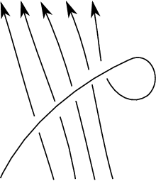
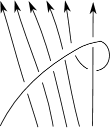
Next, we will consider the diagram below and denote its -th power by . These are required for the satellite construction for links, but we will not need it here.
To conclude this section, we will explain how to actually construct the link diagram in the annulus for a non-reducible singularity. Let be the branches of at and consider truncated Puiseux series
Write and consider the pairs . It is always possible to find a finite truncation of the Puiseux series that does not affect the topological type of the link, so the inductive process we will define is actually finite. For each , let be the set of indices with associated pair . Assume we have an annulus diagram and set
We may assume that , and the link can be represented by the annulus diagram
4.6 Some explicit calculations for the unknot and Hopf link
The following is already apparently known.
Proposition 4.6.1.
For any partition ,
Let be a counterclockwise-oriented diagram. Define the meridian operator on by the construction below:
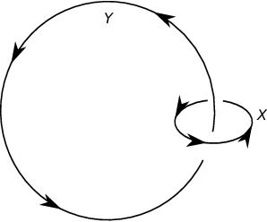
For a partition , the Schur function is an eigenvector for with eigenvalue . Then the HOMFLY polynomial for the colored Hopf link decorated by is simply . In the remainder of this section, we will describe the operator , which is a ring homomorphism . Define the function
Then we have , where for a power series , we write as a polynomial in the and then substitute .
4.7 Behavior of links with respect to blowup
Having discussed the behavior of enumerative invariants with respect to blowups, we need to discuss the behavior of the link with respect to blowing up the origin. Let be the irreducible components of through and denote their strict transforms by . At each point (the exceptional divisor) let denote the singularity of at and be the singularity of at . Choose (truncated) Puiseux expansions
For each of the branches . We may also assume that for all . If we blow up at the origin, consider the chart with coordinates . Substitution, we obtain the new Puiseux expansion
for at . In particular, we obtain the relation
If we perform deeper analysis, we obtain the following result:
Proposition 4.7.1.
If any , then we have
Otherwise, we have
Now we will write down a blowup identity for links. The idea is to use the topological vertex (originally introduced by Aganagic-Klemm-Marino-Vafa) and its relationship with Chern-Sinons invariants of the unknot. For a partition , define
Here, . By the computation of the colored HOMFLY polynomial of the colored unknot (sorry), we obtain the identity
4.8 Relation between PT theory and HOMFLY
We will prove a relationship between the PT partition function for -framed stable pairs in and the HOMFLY polynomial for . We will focus on the simplest case of a node with two branches. The general case reduces to this one by careful checking of what happens on both sides under blowup of at .
Proposition 4.8.1.
We have the identity (possibly up to monomials)
where the superscript low means we take the lowest degree terms.
We only need to prove this for the unknot and the Hopf link.
Proof.
This apparently follows from the fact that the topological vertex calculates both the specialization of HOMFLY of the Hopf link and the stable pairs vertex. See the references to Maulik’s paper for a reference. □
5 Che (Oct 19): Braid varieties and Khovanov-Rozansky homology
5.1 Khovanov-Rozansky homology
Let and be the Cartan. Write , and this has an action of the Weyl group permuting the coordinates. We will specify . We may now define Soergel bimodules
Now define by and by . We may now form the Rouquier complex for a braid as
For example, if , then we have
We may now take the Hochschild homology . We will mostly be concerned with . Continuing our example, we have
We are finally able to define the Khovanov-Rozansky homology
This has gradings for the Hochschild grading, for the internal degree in , and for the homological grading. Continuing our example again, we have
Remark 5.1.1.
We will usually multiply our by as a useful normalization. This is a consequence of us considering instead of .
5.2 Braid varieties
Write for the matrix with s on the diagonal except for a block on the diagonal in the positions. Given , we consider the matrix
Then we may define the braid variety
For example, if for strands, we have
and so
Similarly, for , we have the matrix
and thus we have . Similarly, we may compute
These braid varieties come with a torus action. We would like to write
For example, we have
Doing this on , we obtain an action of on . Continuing our example, we have
Here are some facts:
- 1.
Under mild assumptions, is smooth.
- 2.
If closes to a knot, then the action of is free.
We are now ready to state the main result.
Theorem 5.2.1.
We have an equality
up to a global shift in grading, where is the weight filtration.
5.3 Mixed Hodge Structures
To understand the weight filtration, we will discuss mixed Hodge structures. For a smooth projective variety of dimension , recall the Hodge decomposition
Of course, for general which are not necessarily smooth or projective, this decomposition will fail. In this case, there is a weight filtration
which morally measures how much the Hodge decomposition fails.
Theorem 5.3.1.
Let be a smooth algebraic variety inside a smooth and projective such that is a normal crossings divisor. Write as a union of its irreducible components. Then there exists a spectral sequence
which collapses at the page. Here, is the locus of the -fold intersection.
Note that our spectral sequence looks like
For example, when and , we have , and so we obtain
and for example, .
5.4 Sketch of proof of main theorem
What we will do is to construct a Bott-Semelson variety from the Khovanov-Rozansky homology, then as a fiber over the flag variety we will consider the brick variety of , which is a compactification of .
Definition 5.4.1.
Given , define the Bott-Samelson variety
For example, when , we have
Then . Now we define the open Bott-Samelson variety
We have the projection sending a tuple of flags to . Then we define
where is the Demazure product. Finally, define .
Theorem 5.4.2.
- 1.
, where is with the transpositions reversed.
- 2.
The complement is a normal crossings divisor.
- 3.
The brick variety has a stratification by for subwords of such that .
Remark 5.4.3.
We define for some as
For example, we have . On the other hand, , , and .
Theorem 5.4.4.
As an bimodule, we have
6 Sam (Oct 26 and Nov 09): Finite dimensional type A rational Cherednik representations
Let be the root system, be the Weyl group , and be the -dimensional representation. Sitting inside there is a canonical set of generators.
Definition 6.0.1.
Given a constant , define the rational Cherednik algebra to be the algebra generated by , , and with the relations
- •
;
- •
and ;
- •
,
where and are the canonical set of generators.
This has some induced representations. If is a representation of , then there is an action of on , which is the same vector space. This is given by . Then we may define
Here are some basic properties:
- 1.
There is a grading where have degree , have degree , and has degree .
- 2.
There is a filtration given by taking the total degree in and .
A stranger property is that there is some -triple. Here, if
then is an -triple. This integrates to an action given by , which is called the Fourier transform.
6.1 Relation to KZ-connection
Let and define operators
These are called the Dunkel operators.
Exercise 6.1.1.
If , then this gives the relations in the rational DAHA for .
Corollary 6.1.2.
Because , then a module gives us a bundle with meromorphic connection on . Note that the poles along hyperplanes are of order , which means we have regular singularities and thus we can study representations of DAHA using the Riemann-Hilbert correspondence.
6.2 Background on -representations
The Hecke algebra is a deformation of . Given a parameter , we obtain a parameter . Now there is a theory of Specht-modules.
Theorem 6.2.1 (Dipper-James).
- 1.
There is a flat (over ) family of -modules nduced by any partition of . This exhausts without repetition the representations for not a root of unity and agrees with the usual Specht module for .
- 2.
When is a root of unity, these are not always irreducible. If is the order of and is -regular (the multiplicity of every is less than ), then is irreducible.
- 3.
There always exists a simple quotient of .
- 4.
There is a bijection between blocks of representations of and -cores. An -core is a partition of without -hooks.
For , either is an -core or is one of . In this case, we obtain the representations . Clearly is the trivial representation, , ad is the sign representation.
Proposition 6.2.2.
The composition series of is given by
whenever these are defined. Moreover, , but the other for .
Example 6.2.3.
For , we have the composition series
If we take , the action on has a trivial -dimensional submodule.
6.3 The KZ functor
Consider the weight zero summand of category . Then the monodromy gives us a local system on . Remember that the root hyperplanes were the singularities of our connection . Given , we obtain the module
and in fact this is the monodromy. This gives us a -equivariant local system on , and these are the same thing as . We claim that this gives an equivalence
Proof.
We will give a “proof” of this result. The first thing we need to prove that , where is the monodromy around , where is a small loop around . In the case, our Dunkel operator is simply
For the trivial and nontrivial representation of , we obtain either
But now we may compute the monodromy. In the case of , we have trivial monodromy. In the harder case, if we complexify to and take (corresponding to going halfway around a hyperplane), then we have
This clearly has monodromy because we have the fundamental solution . Then there is something that reduces the general case to this calculation.
This functor factors through torsion because torsion is the kernel of . This was the first step, so this is clear. We now prove equivalence. This follows from the Riemann-Hilbert correspondence once we prove regularity at infinity in some compactification. This computation is omitted. □
We will use
to give a representation of .
Theorem 6.3.1 (BGG (BEG)).
There is a resolution
This result follows from the fact that the block of representations of the Hecke algebra has simple representations, so once we finish at , we must have a torsion module, which must be . If and , then is finite-dimensional.
Example 6.3.2.
By definition, it is clear that . Thus the BGG resolution is the Koszul resolution of . When and , the image is the ideal
where are . These are just two reducible pairs of lines, and so then if we take , we obtain the subscheme defined by the above ideal. Clearly is the ring of functions on this scheme.
In the case, we have is a local complete intersection. This is derived smooth, and so we have some kind of Poincaré duality.
6.4 Characters for representations
Let , where is a basis for and is the dual basis. Then splits as
where acts by . Because commutes with we can keep track of the -grading and -characters.
Definition 6.4.1.
We define
Now we will define the character for . We an -module, we have
Therefore we have
Here, is the lowest weight.
We will now compute for . To begin, suppose that is the trivial representation. Then the lowest weight vector is and the act by . We now have
Next, we use the Koszul-BGG resolution and see that
Finally, we compute the characters for and prove that they exhaust finite-dimensional representations. Suppose is finite-dimensional. For we have . We know that is in the block containing . Therefore we have
This gives us
This is a degree polynomial and also that the trace is finite as , so in fact . Therefore assuming that and is simple. But now we see that , and so
7 Cailan (Nov 09 and Nov 16): Torus knots and the rational DAHA
7.1 Representation theory
We will begin by changing Sam’s formula until it is in the form that Cailan wants:
Definition 7.1.1.
Let be a representation of . Define by
where are the power sums and is the number of cycles of length in .
Remark 7.1.2.
We have . Also, is a basis for , and in fact, there is an isomorphism of Hopf algebras
with the ring of symmetric polynomials in infinitely many variables.
Lemma 7.1.3.
The reflection (representation) of is isomorphic to .
Lemma 7.1.4.
Let be a linear operator and let be a sum of -invaraint subspaces. Then .
Proof.
Clearly is a block matrix. □
Proposition 7.1.5.
For each acting in the reflection representation , we have
Proposition 7.1.6.
For with , we have
Proof.
Note that . Therefore by the previous lemma, we have
By conjugation invariance of the characteristic polynomial, it is invariant under permutation matrices, which corresponds to conjugation in , and so the trace depends only on the cycle type. For each cycle in of length , there exists a -invariant subspace of of dimension . Clearly the trace only depends on the length . Also, we know that
and each is -invariant. Using the lemma again, we have
It is easy to check that , and therefore we have
as desired. □
Theorem 7.1.7.
Let be the graded Frobenius character. This is equal to . Fixing , we claim that the function
satisfies the identity
where .
Proof.
Let . Using Sam’s formula, we have
Therefore
By an easy exercise, it is easy to see that . Therefore we have
Using the fact that , we have
This tells us that
We now have
Remark 7.1.8.
The Frobenius character is really the same information as . For , we see that , and thus . Also, is the generating function for
Theorem 7.1.9.
As a graded -representation, we have
Proof.
It suffices to prove this at the level of the Frobenius character. We have the Cauchy identity
and here we will specialize to
This implies that
Proposition 7.1.10.
We have
Example 7.1.11.
We have .
7.2 HOMFLY polynomial of torus knots
Definition 7.2.1.
We will define the HOMFLY polynomial using the same skein relations as before but with .
Example 7.2.2.
For the trefoil we have .
Definition 7.2.3.
Define to be the quotient of by the relation . Let .
Here, will always be generic, unlike in Sam’s lecture.
Definition 7.2.4.
The Jones-Ocneanu trace is the unique linear map such that , , and for any .
Theorem 7.2.5 (Jones).
Let . Let . Then
Theorem 7.2.6 (Ocneanu).
Let . Then
Proof.
We know that for generic and any satisfying commutativity is a scalar multiple of the trace. □
Definition 7.2.7.
We define to be the closure of the braid .
Remark 7.2.8.
is a knot if and only if . In addition, .
Let .
Lemma 7.2.9.
Fix . Define . Then . Moreover, let and . Then
Proof.
We omit checking that is idempotent. Next, we have a very important fact that is central in . Therefore, for some . By definition, , and so in some basis of , we have
This implies that , and therefore , so , and thus , where is continuous. But now is constant because is connected and is discrete.
We can now thus evaluate at . Note that at , and therefore because , we see that . □
Lemma 7.2.10.
The matrix is conjugate to the matrix for acting on .
Proof.
We know that , and thus is diagonalizable. In particular, the conjugacy class is determined by the eigenvalues and their multiplicities. By the same continuity argument, we can evaluate at . □
Corollary 7.2.11.
Suppose . Then
Proof.
By the lemma, we have
by Galois theory, where are the eigenvalues of . Now everything follows from the Murnaghan-Nakayama rule. □
Theorem 7.2.12.
Suppose . Then
Here, .
Proof.
The only thing left is . By the braid relations, all are conjugate to in , and thus we only need to find the rank of . Note that . Then the rank can be computed in , and so we use the branching rule. There are two irreducibles, where acts by on the trivial representation and by on the sign representation. Therefore and .
This implies that is the multiplicity of the trivial representation , and this is given by . Finally, is given by by the hook length formula (here we specialize ). □
Theorem 7.2.13 (GORS).
The graded Frobenius character of coincides with the HOMFLY polynomial of the torus knot when . Specifically, we have
Proof.
We simply compute
Because , we use some generating function magic to obtain the desired result. □
Corollary 7.2.14 (Rank-level duality).
For , we have
8 Davis (Nov 23): Hilbert schemes, Coulomb branches, and DAHA
8.1 Affine grassmannians
We will begin with some abstract nonsense discussing affine Grassmannians.
Definition 8.1.1.
An -family of vector bundles on the formal disc (or the punctured formal disc ) is a projective finitely generated module over (or ).
These give categories .
Definition 8.1.2.
The affine Grassmannian for a group , denoted is the functor
where is an -family of -bundles () over and is a trivialization of over .
Example 8.1.3.
If , then the set of finitely generated projecive -submodules of such that for some , we have
Remark 8.1.4.
We can define to be those which satisfy the relation for some fixed . Using this, we may view as an -module satisfying some conditions. Therefore, is a closed subfunctor of (which means things inside a -dimensional vector space).
Remark 8.1.5.
Unfortunately, the affine Grassmannian is not a scheme, but at least it is an inductive limit of schemes.
Now consider . This induces an automorphism of the trivial -family of -bundles on , and so there is a natural action
Remark 8.1.6.
We have a simply transitive action on the fiber by , and thus
Example 8.1.7.
Consider the case of . Then the only data that matters is the power of near , and so .
Now we can give a lattice description. Remember that we are considering -stabble subspaces of . This has a basis . But now is a union of points, and so in the increasing limit we obtain .
8.2 Coulomb branches
Definition 8.2.1.
Fix a -representation . We will define the space
where is as before and is a section of over .
This has a subset , where we require to extend to and to extend to a section of . We will call the BFN space, where BFN is Braverman, Finkelberg, and Nakajima.
Definition 8.2.2.
We define the Coulomb branch algebra to be
Example 8.2.3.
Consider and . Then , and then we have .
Example 8.2.4.
Consider and the adjoint representation. If the trivialization is simply , then we need to have no singularities, and therefore . Therefore
and therefore we have
If we modify the second to act with weight , we instead obtain .
Remark 8.2.5.
For , we have , and after localization, this is an isomorphism.
8.3 Hilbert schemes
Definition 8.3.1.
Fix , where is a -representation. Then the generalized affine Springer fiber is defined by
The main claim is the following: Let be a germ of plane curve singularity. Then there is an -generalized affine Springer fiber such that
By the Weierstrass preparation theorem, we assume that . Then as -modules, we can identify . Then if , we can identify the fraction field of with .
Unwinding definitions, points in are the same as -stable, finitely generated, projective -submodules of such that there exists such that
Then we have
We now choose , where corresponds to . We also need . We will also choose such that for some , we have . This implies that
and so . The second condition gives us . By definition of the affine Springer fiber, we only need . This implies that and so we can induct downwards.
Example 8.3.2.
Let . Then -stability is the same as -stability, and so we are looking for something -stable in
which is the same as points. Thus .
Remark 8.3.3.
When , there is another scaling and (called the flavor symmetry). Then we have an action of , and so . If we denote the group by , then we define to be the stabilizer of , and this is isomorphic to . By some general theory, there is an action of on . We claim that for , is the spherical rational DAHA.