D-modules and localization
Geometric Representation Theory Learning Seminar
Spring 2022
Notes by Patrick Lei
Lectures by Various
Columbia University
Disclaimer
These notes were taken during the seminar using the vimtex package of the editor neovim. Any errors are mine and not the speakers’. In addition, my notes are picture-free (but will include commutative diagrams) and are a mix of my mathematical style and that of the lecturers. If you find any errors, please contact me at plei@math.columbia.edu.
Seminar Website:
https://math.columbia.edu/~plei/s22-GRT.html
1 Fan (Feb 09): D-modules, bare minimumz, part 1
For now, let be a smooth affine variety over .
Definition 1.0.1.
A differential operator of order is a -linear such that for any , is a differential operator of order . In other words, for any , we have
We will call the set of differential operators of order . We will see later that , , and . Some other facts are:
- •
is generated by under the rules
- •
For any , .
We will now prove these facts. First, by and . On the other hand, we note that is given by and .
Lemma 1.0.2.
We have and .
Proposition 1.0.3.
There is a canonical map .
On one hand, note that . Taking symmetric powers of this, we obtain a map .
To define the inverse, note that we have a morphism in degree already. Inductively, we consider the map
This kills , so it descends to . Inductively, we use the adjunction to obtain
It is easy to check that this is an inverse.
We will now consider generation of by and . We will endow with the Lie bracket
We will show that
Clearly there is a map , whose source we call . The commutation relations imply that is commutative, so we have a surjection
Clearly, we see that is an isomorphism, so is an isomorphism.
Finally, consider the map given by
Clearly this is well-defined, so it suffices to check that is an isomorphism. But both sides are , and by exactness of localization we are done.
Now that we have a sheaf , we will define -modules.
Definition 1.0.4.
A left -module is a quasicoherent sheaf with a left -action.
Example 1.0.5.
Clearly and are -modules. On the other hand, if is the skyscraper sheaf at , then is a right -module.
Proposition 1.0.6.
Let . Then
- •
is a left -module with the formula
- •
is a left -module by
The analogous statement is true for right modules.
- •
If is a right -module, then is a right module by
- •
is a right module by
Recall that acts on by the Lie derivative. Then admits a right -module structure by .
Definition 1.0.7.
Define the right -module by
Now if is a left -module, then we see that
is a right -module. Now if is a right -module, then
We will call this sheaf .
Proposition 1.0.8.
The functors and give an equivalence of categories between and .
Proof.
We will prove an adjunction
This will be defined by
Here, we note that , so we have the adjunction. We only need to check that the unit and counit are isomorphisms now. Here, we have
and the unit is similar. □
2 Fan (Feb 16): D-modules, bare minimumz, part 2
Our goal is the following underived theorem:
Theorem 2.0.1 (Kashiwara).
Let be a closed immersion. Then there exist functors
giving an equivalence of categories.
Definition 2.0.2.
Let be a morphism. Then the -module pullback is defined by
with the -action given by
2.1 Transfer modules
Definition 2.1.1.
Define the transfer module .
Now that we have this definition, it is clear that .
Definition 2.1.2.
Define the functor by
After symbol pushing, we obtain
This motivates the following definition:
Definition 2.1.3.
Define the other transfer bimodule by
Now we have .
If is a closed immersion, then is right exact. We hope that an adjoint exists, and in fact we will define a candidate.
Definition 2.1.4.
Define the functor by
Example 2.1.5.
Let be a local étale coordinate system on . Then write . Now we define
This is an anti-homomorphism of . Defining a right action on by , this is the left-right flip.
Example 2.1.6.
Now let be a coordinate system on and suppose is cut out by . Then we have
On the other hand, we have .
2.2 Proof of Kashiwara
We will first prove an adjunction. In fact, we will prove the adjunction on the level of sheaf Homs. But this reduces to
There is a natural morphism coming from , so we only need to check locally that this is an isomorphism. But now the left hand side becomes
where is the subsheaf with supports in (note notation is different from Hartshorne).
We will now prove that the units and counits are isomorphisms. We can do this affine locally, so we will choose an étale coordinate system on . We will assume that , and in particular we can reduce to the case where . We will simply write for simplicity. First, consider
This is determined by such that . Write . Because , we have and . Now we have
This is nonzero unless for all , so .
Now consider
Locally, the left hand side is simply . Consider the operator . Then define . We now have
and
so we see that act like shift operators. Now define . Then we will show that . To show this, we will use induction. If , then , so . For the inductive step, we note that if , then
Thus . Then
so , and thus
Because is supported on , we have , and thus
But now is determined by and must be killed by , so .
3 Fan (Mar 02): D-modules, bare minimumz, part 3
Recall that we have an underived version of Kashiwara. We will prove that
Proposition 3.0.1.
If a -module is coherent over , then it is locally free over .
Also, we will prove
Proposition 3.0.2.
Let be a smooth closed subvariety. Then there exists a functor such that .
Finally, we will prove
Theorem 3.0.3.
There exists a functor such that give an equivalence of categories.
3.1 Proof of first proposition
Note that local freeness can be checked at stalks. Also, flatness can be checked at stalks. Over local rings, flat is equivalent to free. Finally, for finite modules over a reduced Noetherian ring, flatness is the same as the rank of being locally constant. Then, any two closed points on a smooth variety can be connected by (a chain of) smooth curves. Therefore, we can reduce to the case when is a smooth curve.
First, we will show that is torsion-free. If has torsion at , then there exists supported at , so by Kashiwara, there exists such that
which is not coherent. But now is not coherent. Now because is smooth, is a DVR, and in this case, being torsion free is the same as being free.
3.2 D-modules on singular varieties
Now suppose is singular and affine. Choose , and then define to be , and this automatically satisfies Kashiwara. This is compatible with diagrams of the form
We will not consider singular things, so we will not need this in the future.
3.3 Construction of functors
We will define the functors we want to study. First define by
where the shift apparently makes the Riemann-Hilbert correspondence more convenient.
On the other side, define by
Theorem 3.3.1 (Bernstein).
Let be separated and Noetherian. If is a sheaf of -algebras, quasicoherent as an -module. Let be those with quasicoherent cohomology. Then
is induced by the inclusion of quasicoherent modules into all modules.
Example 3.3.2.
If is an open embedding, then is exact and is precisely , so in fact . Also,
and therefore , and thus .
Example 3.3.3.
Let be a closed embedding. Choose coordinates of such that is cut out by . Then we know
wnere is a resolution of -modules. Note that
and that
Applying , we obtain a resolution
of locally free -modules. Therefore we have
On the other hand, is locally free as a right -modules, so .
3.4 Proof of second proposition
First, we will show that . But it suffices to see that . Now it suffices to show that
Note that has rank , so there exists a canonical pairing such that
Therefore
Comparing this to
we have the desired result.
Next, we will show that in . Recall from the proof of Kashiwara that
We will prove the derived version of this. Note that is exact, so it sends injectives to injectives. We now claim that the map
induced from is an isomorphism. This is by an exact triangle
It suffices to show that . But this is because
By vanishing of , we are done.
3.5 Proof of Theorem
Finally, the proof of the derived version of Kashiwara follows from the underived version by an inductive argument using truncation functors, which is not reproduced here.1
4 Fan (Mar 09): brief interlude: refresher on algebraic groups
We will call the general linear group, the upper triangular matrices, the nilpotent part, and the maximal torus.
Example 4.0.1.
Here are some examples of group schemes. First, we have , whose functor of points is . Analogously, we have which has functor of points .
Proposition 4.0.2 (Cartier).
In characteristic , all algebraic groups are smooth.
Proposition 4.0.3.
For algebraic groups, smooth is the same as geometrically reduced.
It should be clear what it means to be a sub-group scheme and a normal sub-group scheme. In fact, if is an algebraic subgroup, the inclusion is a closed immersion.
Proposition 4.0.4.
For algebraic groups, connected is the same as being irreducible.
For a homomorphism of algebraic groups , we have a kernel. Then
is exact if maps isomorphically to the kernel of and is faithfully flat. In fact, any factors as into a faithfully flat map followed by a closed immersion. As one would expect, we can construct stabilizers of when acts on . As a special case of this, we can construct normalizers and centralizers of subgroups.
Example 4.0.5.
Some other classical examples of algebraic groups are given by
- •
;
- •
.
- •
.
- •
.
Of course tori are defined to be .
Definition 4.0.6.
Suppose are smooth and connected with . Then is an isogeny if is a finite algebraic group. In general and are isogenous if they are connected by a zigzag of isogenies.
Theorem 4.0.7.
An algebraic group is affine if and only if is a closed subscheme of .
We will define to be the functor , and a representation is a morphism .
Definition 4.0.8.
Let be a subgroup. Then is -invariant if is the same as . Then is a quotient of by if is faithfully flat, is -invariant, and if
is an isomorphism.
All quotients exist and are quasiprojective varieties. If is a normal subgroup of , then is also an algebraic groups. If are affine and is a normal subgroup, then is also affine. Note tha this fails for not normal, because is always projective.
Definition 4.0.9.
A filtration or a subnormal series is a sequence
A composition series is a filtration where For composition series, the quotients are unique up to reordering and isogeny.
Definition 4.0.10.
Define . Then the derived series of is .
Definition 4.0.11.
A subgroup is solvable if . Equivalently, there exists a filtration with abelian quotients.
Definition 4.0.12.
A group is unipotent if every representaiton has a fixed vector. Equivalently, is isomorphic to a subgroup of .
Definition 4.0.13.
Let be a smooth connected linear algebraic group. Then the radical is the maximal smooth connected solvable normal subgroup. In addition, the unipotent radical is the smallest unipotent normal subgroup. is semisimple if and is reductive if .
Theorem 4.0.14 (Jordan decomposition).
For , there exists a unique such that
- 1.
If , then is semisimple (diagonalizable after field extension) and for some .
- 2.
This decomposition is functorial under .
Definition 4.0.15.
A group is diagonalizable if is isomorphic to a subgroup of . Equivalently, is spanned by such that (grouplike elements).
Proposition 4.0.16.
There exists an equivalence of categories between the opposite category of finitely-generated -modules and diagonalizable algebraic groups given by and .
Definition 4.0.17.
A group is of multiplicative type if for some finitely generated abelian group .
Having defined the characters , we can define the cocharacters
Definition 4.0.18.
Let . If there is an extension , then we can define . For , we have an action of on by conjugation. Then we can define
These are all subgroups of .
Note that an action of on induces a decomposition
Then corresponds to positive weights, corresponds to nonnegative weights, and corresponds to the weight subspace.
Proposition 4.0.19.
In characteristic , unipotent algebraic groups are the same as finite-dimensional nilpotent Lie algebras.
Definition 4.0.20.
A group is trigonalizable if is isomorphic to a subgroup of . Equivalently, every irreducible representation is finite-dimensional. Also, this is the same as being an extension of a diagonalizable group by a unipotent group.
Theorem 4.0.21 (Lie-Kolchin).
(Split) solvable implies trigonalizable. In fact, for smooth connected groups over an algebraically closed fields, the two conditions are equivalent.
Definition 4.0.22.
A Borel subgroup of a group is a maximal smooth connected solvable subgroup.
Borels are minimal parabolic subgroups. We then have . We also have and . We define to be the Weyl group. Also, all pairs of a Borel and a maximal torus are conjugate to each other. For reductive, we have
The quotient is semisimple. For example, , which is isogenous to .
5 Fan (Mar 23): localization: d-modules and representationZ
We will warn that the things that we say may be slightly wrong because every source uses a different convention. Here, localization will take the form
where the -modules live on and everything is twisted in some way. The three ways to get the are by:
- 1.
Using line bundles to twist ;
- 2.
Doing something like ;
- 3.
Taking some quotient of as a Lie algebroid.
All of these strategies are the same.
Definition 5.0.1.
A sheaf on is -equivariant if, considering , we equip with an isomorphism
such that
- 1.
;
- 2.
We have the commutative diagram
on .
5.1 Universal enveloping algebras
Recall that a central character is the same as a -orbit (by the dot action) on by Harish-Chandra. Then we define
Now let be the -th infinitesimal neighborhood of the identity. Then for an open set , we obtain a sequence of morphisms
This is the same as the data of a map
Therefore, we have a morphism . This satisfies for all the identity
and in particular .
Definition 5.1.1.
A Lie algebroid is a sheaf isomorphic to extending such that
The corresponding construction for the universal enveloping algebra is with a product extending that of such that
Now extends to . We can also write . Here, we have
Then for , points of are the same as choices of a Borel subgroup . We can similarly define . For all , we have
In particular, we have a .
Now we may define
This is in fact a two-sided ideal, and so we define
In this perspective, we have a natural projection and a natural sequence .
5.2 Line bundles
Let be a module over . Then define on by
Then we have a projection . When is actually a representation of , then . Then for a character , we can define
Definition 5.2.1.
An -twisted differential operator of order is such that for any , we have . The sheaf of such twisted operators is called .
Proposition 5.2.2.
For any , we have .
Theorem 5.2.3 (Beilinson-Bernstein localization).
There are equivalences of categories
whenever is regular and dominant.
5.3 Taking -invariants
Definition 5.3.1.
A weakly -equivariant -module is a -module that is -equivariant as a quasicoherent sheaf such that the morphism
is -equivariant.
Consider the map , which acts on . Then we define . This is in fact a Lie algebra homomorphism to .
Definition 5.3.2.
A -module is strongly -equivariant if .
We now define the sheaf , which is weakly -equivariant and has . We will denote the category of weakly -equivariant -modules with by . To relate all of the notions we have defined so far, we have
In this situation, localization becomes
Theorem 5.3.3.
We have an equivalence of categories
6 Fan (Mar 30): proof of localization: d-modules and representationz, part 1
6.1 An example with
Let be a module over and consider . We will see that
Here, is the map with weight . We will consider the case when and thus .
If we set , then we see that
But this implies that , and a similar result is true for . Therefore,
Doing more computations, we note that the action of acts on , and in fact we obtain . We also have an action of on . On the chart , we have
and we have on and on . For the element , we note that
on and on . Therefore we have
Now we know that . Taking global sections, consider the basis . Then we see that , and this is the representation .
6.2 Main results
There are a few key results:
Theorem 6.2.1.
We have the identity
Theorem 6.2.2.
- 1.
If is -antidominant, then
is exact.
- 2.
If is -regular, then is faithful.
Theorem 6.2.3.
For the action of on , then
The logical equivalences are that the first two theorems imply localization and that the third implies the first. Also, Kostant implies the third theorem.
6.3 Proof of localization
Let be a quasicoherent sheaf of algebras on and . Then and give an equivalence between -modules and -modules. It is clear that is an isomorphism to all free because . But then for any , if we consider a presentation
and note that are isomorphisms and the sequence stays exact after applying , we see that is an isomorphism.
To prove that the counit is an isomorphism, note that is conservative, so it suffices to show that is an isomorphism. But here we have
so is an isomorphism.
6.4 The technical results
Next, note that if is a -module for , then because
Proposition 6.4.1.
The map factors through .
Proof.
Let . It suffices to show that
is the zero map. For , note that
The action of on this is actually .
By the discussion from last semester, in the diagram
is independent of the choice of Borel. Also, because acts on by , on by , and therefore, taking the transpose, acts on , and acts by . □
Lemma 6.4.2.
The inclusion induces an isomorphism .
Third theorem implies first theorem.
Note that inherits the filtration from and consider the map . It suffices to show that the graded version of this is an isomorphism. Here we have a sequence of maps
whose total composition is an isomorphism. Here, the second map is , the third map comes from something like
and using left exactness of . Finally, factors through . □
7 Fan (Apr 06): proof of localization: d-modules and representationz, part 2
7.1 Comments on equivariant things
Let act on . Recall the definitions of weakly -equivariant and strongly -equivariant -modules.
Proposition 7.1.1.
Suppose is a principal -bundle. Then there is an equivalence between -modules and strongly -equivariant -modules given by and .
Proposition 7.1.2.
We have an equivalence .
Proof.
In general, if is a quasicoherent sheaf on , is -equivariant because the diagram
commutes. We also need to check compatibility with the -action, which means that
commutes. Here, we are assuming that is locally in the Zariski topology (this is true in the cases we are interested in), so . Now locally has trivial -equivariant structure and is strongly -equivariant by definition, so is also strongly equivariant.
Next, it is clear that
This implies that our assignment is fully faithful. Now for a strongly equivariant -module , we can write for some on . Finally, we check that
7.2 Proof of Theorem 6.2.2
First we will prove exactness. It suffices to show that
is exact. However, we identify the first term with , and then global sections take us to . This lands inside a non-finitely generated version of category , and then we take to get a vector space. But now
This is exact exactly when is a projective Verma module, which follows from our assumptions on .
Definition 7.2.1.
A sheaf of twisted differential operators is a sheaf of -algebras with a filtration such that
- 1.
induces ;
- 2.
The natural map is an isomorphism;
- 3.
The map given by is an isomorphism.
Note here that is a sheaf of twisted differential operators. This is because the image of in is , so we get an exact sequence
Next, the image of in is , so we have
The next fact is that for any , . To see this note that is -equivariant, so the map
factors through because acts on by for any .
Finally, we will accept as fact that , that , and if , then
Let . Here, we have
Now we are ready to prove faithfulness. Let . We want to show that . Let , where . Now if is the maximum length in the Weyl group, consider
consider the filtration
Now if is the inclusion, we have an exact triangle
which gives us an exact sequence
and in particular, we obtain
The upshot is that we have a filtration of such that
Now we have a spectral sequence
But now the page is actually
8 Fan (Apr 13): some more on D-modules and identifying some highest-weight modules in the setup
We will discuss important notions like coherence, holonomicity, duality, and then identify the -modules corresponding to important modules in representation theory under localization.
8.1 Coherence and holonomicity
Definition 8.1.1.
A filtration for is compatible with if
Definition 8.1.2.
A good filtration of satisfies one of the following conditions:
- •
is coherent as a -module;
- •
is a coherent -module for all and for all sufficiently large .
Definition 8.1.3.
Define the singular support , where we take any good filtration on . This is in fact independent of the good filtration.
Proposition 8.1.4.
A -module is -coherent if and only if it has a good filtration.
Theorem 8.1.5 (Bernstein’s inequality).
Let be a nonzero coherent -module. Then
Proposition 8.1.6.
Let be a closed embedding. For every , . In addition,
If is an open embedding and , . In addition,
Another fact is that if , in fact .
Definition 8.1.7.
is holonomic if the inequality in Bernstein’s inequality is in fact an equality, that is if
Define and to be the categories with holonomic and coherent cohomology, respectively.
Theorem 8.1.8.
Let . Then preserve .
Now consider the duality functor given by
Fortunately, we can compute this by taking a projective resolution, so
Theorem 8.1.9.
If is holonomic, then is concentrated in degree , and so is a duality functor on holonomic -modules.
This allows us to construct a six functors formalism for -modules. Define the pushforward with compact support
and the pullback
Theorem 8.1.10.
This, combined with the existing , form a six functors formalism. In addition, the natural map is an isomorphism if is proper and if is smooth.
8.2 Representation theory
For any subgroup , define a -module to be a module where the action of comes from differentiating an action of . Then we obtain
Sticking to , define and . Then denote their images under localization by .
Now consider the inclusion . Define
Lemma 8.2.1.
- 1.
;
- 2.
There is no nontrivial submodule of supported on .
Proof.
Define
These give algebraic groups . For , choose a lift of and define
Note that . We now have a diagram
Then we compute
We then have
because
so we obtain
If we let act on by , this becomes an isomorphism of -representations, and so we can compute the characters. First, we have
Next, we obtain
The action of on has weight
so . In total, the character is
We now prove the second part of the lemma. Let and . We have an exact triangle
and because , we see that . □
Proposition 8.2.2.
We have
Proof.
Induct on . First, for , if for all , then . To see this, consider the map . If this is not surjective, then there exists a morphism and thus is a Jordan-Holder factor of . But then is a Jordan-Holder factor of , so . this gives a nonzero map .
By the inductive hypothesis, , so for all . Because is supported on , which does not intersect , by adjunction we see that for all supported inside . Applying global sections, we see that . □
One can also show that is the image under of . This is very difficult and uses the Riemann-Hilbert correspondence. Also, .
9 Kevin (Apr 20): the Riemann-Hilbert correspondence
Note: these are the speaker’s notes. Minor modifications were made to adapt to my typographical style choices. Some references include Hotta-Takeuchi-Tanisaki (D-Modules, Perverse Sheaves, and Representation Theory, Part I), Dimca (Sheaves in Topology, Chapters 4-5), and Borel (Algebraic D-modules).
9.1 Review of constructible sheaves
Since Caleb’s talk last Friday covered this material and (presumably) most of you were there, I’ll briefly review constructible sheaves and the six functor formalism.
Let be a complex variety. A stratification of is a locally finite partition , where each is a smooth connected locally closed subvariety such that each is a union of strata. A -sheaf on is constructible (with respect to this stratification) if is a local system with finite-dimensional fibers for each . A complex is constructible (with respect to this stratification) if each cohomology sheaf is. We use to denote the full subcategory of consisting of constructible complexes.
Why consider constructible sheaves? Local systems are all over the place, but they aren’t well-behaved under the usual sheaf operations. Constructible sheaves are. Here are the six operations we can perform (let’s say we have a map ). All the operations are derived, so we will omit the and for the most part.
- •
- •
- •
- •
- •
- •
We have adjunctions . Moreover, there is a Verdier duality functor such that . Here, is the dualizing sheaf, which is ( is the dimension of ) when is smooth. intertwines the functors: , .
9.2 The Riemann-Hilbert correspondence for integrable connections
For the remainder of this talk, all varieties will be smooth, since we want to talk about D-modules.
Let be a smooth variety. The Riemann-Hilbert correspondence (for varieties) is an equivalence (here, stands for regular holonomic; I will define this shortly). To motivate the general correspondence, we will first discuss the simplest case: integrable connections. Let be an integrable connection, i.e. a vector bundle with a flat connection. We can get a local system whose sections are horizontal sections of , i.e. sections for which . This produces an exact functor from the category of integrable connections on to the category of local systems on : .
Is this functor an equivalence? If we consider the analytic analogue (we consider flat holomorphic connections on the complex manifold ), the answer is yes: is an equivalence. When is proper, the answer is yes by GAGA. However, in general, in the algebraic case, this functor is not necessarily an equivalence, as the map is not necessarily an equivalence. We would like to apply GAGA; to do this, we must restrict to the subcategory of regular integrable connections on , which are connections that behave well near the boundary of a compactification .
We first define regularity for connections on a curve. A smooth curve can be compactified to a smooth proper curve by adding a finite number of points. Let , and let be an integrable connection on . Letting be the inclusion, we get a meromorphic connection on with possible poles at . Let , let denote the fraction field of , and let be a local parameter at . Taking the stalk of at , we get a -vector space with a connection . We say that is regular at if either of the following equivalent conditions holds:
- •
(Algebraic) There exists a finitely generated -submodule such that and .
- •
(Analytic) All locally defined horizontal sections of (local in the analytic topology) grow at most as fast as for some as .
We say that is regular if the meromorphic connection is regular at all .
One way to make sense of the algebraic condition is to pick an basis of and work analytically. In terms of this basis, the set of conditions for horizontal sections of near is a set of ODEs
where the are some meromorphic functions defined near (these form the connection matrix). The condition means that is holomorphic for all . This translates to the condition about moderate growth. For instance, the ODE has solution for and for . When , the solution is a meromorphic function with moderate growth. When , has an essential singularity at and, in particular, doesn’t have moderate growth.
Now consider a smooth variety of any dimension. By resolution of singularities, we can find a smooth compactification such that is a divisor. We say that an integrable connection on is regular if for every map from a smooth curve , the induced integrable connection is regular. It can be shown that this notion is independent of choice of . For the complex manifold , we can similarly define regular integrable connections as certain meromorphic connections on with respect to , except that we consider maps from the unit disc such that . Unlike the algebraic case, analytic connections on don’t have unique meromorphic extensions to , so it doesn’t make sense to say that a particular integrable connection on is regular.
Here’s a big theorem of Deligne, known as Deligne’s Riemann-Hilbert correspondence.
Theorem 9.2.1 (Deligne).
The restriction defines an equivalence of categories
Corollary 9.2.2.
The functor
is an equivalence.
Sketch of proof.
After picking a compactification with divisor boundary , we can factor this functor as
The functor is an equivalence because algebraic connections on extend to unique meromorphic connections on with respect to . The functor is an equivalence by a GAGA argument; here, we need regularity because GAGA only applies to coherent sheaves on . The functor is an equivalence by the preceding theorem. We’ve already noted that the functor is an equivalence.
□
Deligne’s Riemann-Hilbert correspondence provides an algebraic description of the category . The Riemann-Hilbert correspondence of Mebkhout and Kashiwara does the same thing for .
9.3 The Riemann-Hilbert correspondence for regular holonomic D-modules
Recall that a coherent D-module is holonomic if its characteristic variety has dimension , where is a good filtration. We can define the characteristic cycle of a holonomic -module as the formal sum over the irreducible components of . Since is conic Lagrangian, any irreducible component must be of the form , where is a smooth locally closed subvariety of .
For a short exact sequence of holonomic D-modules
. Moreover, iff . Thus, holonomic D-modules have finite length. The simple holonomic D-modules are the minimal extensions , where is a smooth locally closed subvariety such that is affine and is a simple integrable connection on . This means that we can think of holonomic D-modules as D-modules built from integrable connections, in the same way that constructible sheaves are built from local systems. , so tells us where the composition factors of are supported.
We say that a holonomic D-module is regular holonomic if for all its composition factors are of the form for a regular integrable connection on . We let (resp. ) denote the full subcategory of consisting of complexes with holonomic (resp. regular holonomic) cohomology sheaves. To get a constructible complex from a holonomic complex , we apply the de Rham functor . Concretely,
where is in degree 0. Here, if we pick local coordinates , the map sends .
Theorem 9.3.1 (Kashiwara’s constructibility theorem).
For , .
Theorem 9.3.2 (Riemann-Hilbert correspondence).
The functor is an equivalence respecting the six functor formalism on each category. The natural t-structure on corresponds to the perverse t-structure on .
We can also do this with the solution functor defined by . The de Rham and solution functors are related by .
When is an integrable connection on , is the de Rham complex of with differential . By the holomorphic Poincaré lemma, is quasi-isomorphic to the local system of horizontal sections of in degree (and is the dual local system in degree ). This matches our expectation from the Riemann-Hilbert correspondence for integrable connections.
10 Kevin (Apr 27): the Kazhdan-Lusztig conjectures
Note: These are the speaker’s notes. Minor modifications were made to adapt to my typographical conventions. Some references include Yi Sun’s notes “Perverse sheaves and the Kazhdan-Lusztig conjectures” and de Cataldo-Migliorini’s notes “The Decomposition Theorem, perverse sheaves and the topology of algebraic maps.”
10.1 The Kazhdan-Lusztig conjecture
I gave this talk last semester, but I forgot everything, so here it is again, possibly with different conventions. The Hecke algebra of a Weyl group is the -algebra with -basis for and multiplication given by and relations
carries an involution given by and . There is a special basis () of satisfying the given properties:
- •
.
- •
with of degree for and .
The Kazhdan-Lusztig polynomials describe the change of basis matrix from to . The Kazhdan-Lusztig conjecture states that these polynomials describe the change of basis matrix from the Verma modules to the simple modules in :
10.2 Sheaves on the flag variety
To prove the Kazhdan-Lusztig conjecture, we translate everything to sheaves. Let (resp. ) be the Schubert cell (resp. Schubert variety) corresponding to , and let denote the inclusion.
We have the following functors from the last couple talks:
- •
Beilinson-Bernstein localization .
- •
The Riemann-Hilbert correspondence . I haven’t defined the category of perverse sheaves , so here it is. is the full subcategory of consisting of complexes such that
is the heart of the perverse t-structure, so it is naturally an abelian category. Examples of perverse sheaves include intersection cohomology complexes, which we will define shortly.
It can be shown that maps to , so that we can consider the image . It is possible to upgrade and to functors on categories of -equivariant sheaves, so that the image is contained in the subcategory of constructible with respect to the Schubert stratification of . We are concerned with the images of the Vermas and simples in . Fan showed two weeks ago that
Since commutes with the six functors, we have
Implicitly, here we are using the fact that is an affine locally closed embedding, so that and are exact functors (both for the ordinary t-structure on regular holonomic D-modules and for the perverse t-structure on ). We’ll abuse notation by writing for the sheaf on .
10.3 Categorification of the Hecke algebra
The Kazhdan-Lusztig conjecture predicts the change of basis matrix for two bases of . Having done all this geometric work, we have shown that this is the change of basis matrix for two bases of (here, is the full subcategory of complexes constructible with respect to the Schubert stratification). We can rephrase the Kazhdan-Lusztig conjecture purely in terms of sheaves:
Theorem 10.3.1 (Kazhdan-Lusztig conjecture).
In ,
Figuring out the change of basis matrix amounts to figuring out the stalks of along the Schubert cells. For a complex of sheaves on constructible with respect to the Schubert stratification, let
Here, is the dimension of any stalk of along .
Theorem 10.3.2.
To prove the theorem, we’ll show that perverse sheaves categorify the Hecke algebra: will correspond to , whereas will correspond to . It’ll be convenient for us to work with rather than . Just as the Bruhat decomposition gives us a stratification of by -orbits, we get a stratification of by -orbits, where acts diagonally. We have , where is the -orbit of . The projection (resp. ) is a Zariski fibration with fiber (resp. ). Thus, , where . Thus, , and for a complex of sheaves on constructible with respect to the decomposition into -orbits (we’ll call this the Schubert stratification as well), define
By the above observation, , so we’ll want to show that .
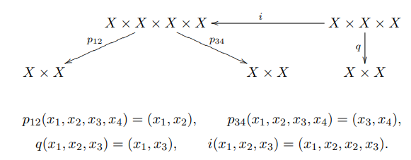
We’ll need an operation on sheaves to correspond to the multiplication on the Hecke algebra. Let be the full subcategory of complexes constructible with respect to the Schubert stratification such that either for all odd or for all even (this is called parity vanishing). Given , we can define the convolution to be , where the maps fit in the following diagram that I’ve stolen from de Cataldo-Migliorini:
Proof of Theorem 10.3.2.
We’ll prove Theorem 10.3.2 by induction. The base cases consist of and for a simple reflection . We have , so , and . is a Zariski fibration with fiber , so is smooth of dimension , and . The Schubert stratification gives , so . In particular, .
To induct, we’ll show that convolution with corresponds to multiplication by in the Hecke algebra.
Lemma 10.3.3.
For , . In particular, .
Proof.
This is proven by a direct computation. We have
so
Let be a point of . Then . Let denote this . Then . By constructibility on , is constructible with respect to , where and is a point. Because is contractible and is a complex with locally constant cohomology, each is a constant sheaf, and . The decomposition gives us a long exact sequence in compactly supported cohomology . By parity vanishing, this long exact sequence splices into short exact sequences . Poincaré duality tells us that for any . Thus, .
To finish, we must identify which strata of contain and . If , then , and , so that . If , then , and , so that . This turns out to be the formula for multiplication by .
□
To finish the proof, we must compute the remaining . Unlike the , might not be smooth, so might not just be a shifted constant sheaf. To compute , we apply the decomposition theorem to the Bott-Samelson resolution . For a reduced expression , we define . is smooth because is a -fibration. is defined by ; this is an isomorphism over , so it is a resolution of singularities.
By definition, . Thus, by Chapter 10.3.3, . Since is smooth, , and the decomposition theorem (which I will not state or explain) states that is a direct sum of shifted ’s: for some finite-dimensional -vector spaces . Since is a direct summand of , . Applying , we have , where . Since is self-dual and is proper, , and . This implies that .
By induction on length, we have . Since everything on the RHS is self-dual in , must be self-dual. It remains to see that if we write , then (1) , (2) , and (3) :
- (1)
This follows from the fact that .
- (2)
This follows from the equation , as the first term contributes and no other terms contribute any.
- (3)
This follows from the support condition on : if . Since , this says that . Thus, , as desired.
By the uniqueness of the Kazhdan-Lusztig polynomials, , and , as desired.
□
To finish the proof of the Kazhdan-Lusztig conjecture, for , we define . By parity vanishing (in particular, only when ),
We have . From these computations, we see that is an isomorphism of -modules. Since , we see that in , which is exactly what we want.